Average required income for Troutdale detached homes declined from $137,475 in 2024 to $131,873 in 2025. While required incomes fell only modestly, affordable detached-home sales increased dramatically as many homes sat near the affordability threshold. Rates tipped the scale.
Troutdale arch sign. Photo: Abdur Abdul-Malik, Portland Appraisal Blog
The amount of income required to purchase a detached home in Troutdale declined modestly between 2024 and 2025. While average and median required incomes fell by roughly 4%, the share of detached-home sales classified as affordable under the Portland Appraisal Blog Affordability Index (PABAI) increased dramatically.
The table below compares key required-income metrics across both years.
Metric
2024
2025
Change
Avg Required Income
$137,475
$131,873
-4.07%
Median Required Income
$134,148
$128,256
-4.39%
Affordable Sales
7
43
+36 homes
% Affordable
6.25%
34.96%
+28.71 pts
Detached-home affordability overview, Troutdale city limits. Affordable homes determined using PABAI. Single-Family Detached Residential | 2024 vs. 2025 Data: RMLS |PortlandAppraisalBlog.com
How “affordable” is defined: PABAI calculates the income needed to buy each home using its actual reported price, taxes, HOA dues, and insurance estimate, financed at the Freddie Mac 30-year rate in effect at the time of sale. A home counts as affordable if that required income is at or below the HUD median family income for the Portland-Vancouver-Hillsboro MSA in effect at the time.
At first glance, the affordability gains appear out of proportion to the decline in required incomes. Average required income fell just 4.07%, yet affordable detached-home sales increased from 7 to 43.
Part of the explanation can be found in how ownership costs were allocated.
Category
2024
2025
Change
Avg Principal & Interest Share
82.47%
82.05%
-0.42 pts
Avg Taxes Share
12.01%
12.17%
+0.16 pts
Avg HOA Share
0.21%
0.41%
+0.20 pts
Avg Insurance Share
5.31%
5.37%
+0.06 pts
Average share of housing payments attributable to principal & interest, property taxes, HOA dues, and insurance as modeled under the PABAI framework. Shares are averaged across all detached sales; sales without HOA dues count as 0% HOA. Single-Family Detached Residential | 2024 vs. 2025 Data: RMLS |PortlandAppraisalBlog.com
Mortgage principal and interest accounted for roughly 82% of the typical modeled housing payment in both years. While the P&I share declined by only 0.42 percentage points between 2024 and 2025, that small change proved meaningful because detached-home sales were heavily concentrated near the affordability threshold. In a market sitting at the boundary of affordability, even modest improvements in financing costs can move a significant number of homes from unaffordable to affordable.
Taxes and insurance remained relatively stable. HOA dues represented a larger share of modeled ownership costs in 2025, although part of that increase can be attributed to a greater number of HOA-governed homes selling in 2025 (35) than in 2024 (24).
The table above illustrates why mortgage rates matter. When more than four-fifths of a typical housing payment is attributable to financing costs, even modest improvements in mortgage financing conditions can materially affect affordability.
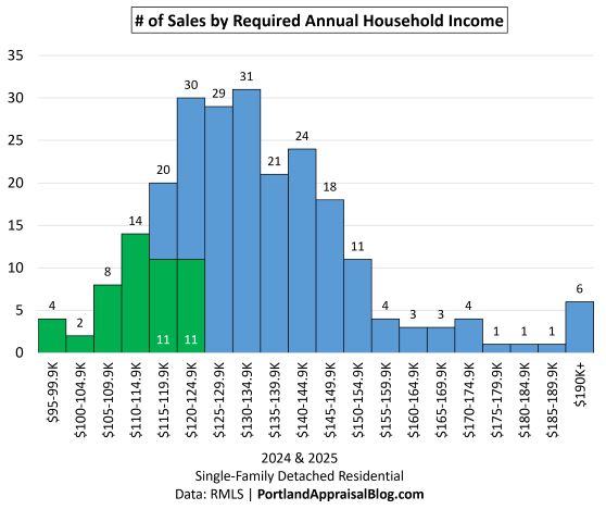
The chart below combines 2024 and 2025 detached-home sales to show where required incomes were concentrated.
Most detached-home sales required between roughly $115,000 and $149,999 of annual household income. The green bars represent homes that met the PABAI affordability standard in effect at the time of sale.
The first four income bands were naturally affordable because they generally fell below the applicable HUD median family income thresholds throughout the study period. Additional affordable sales appeared in the $115,000-$119,999 and $120,000-$124,999 income bands, reflecting changes in affordability thresholds and financing conditions over time.
The table below summarizes the distribution and includes the percentage of sales in each band, making it easier to evaluate where the market was concentrated.
Required Income
# of Sales
% of Sales
# Affordable
$95-99.9K
4
1.70%
4
$100-104.9K
2
0.85%
2
$105-109.9K
8
3.40%
8
$110-114.9K
14
5.96%
14
$115-119.9K
20
8.51%
11
$120-124.9K
30
12.77%
11
$125-129.9K
29
12.34%
0
$130-134.9K
31
13.19%
0
$135-139.9K
21
8.94%
0
$140-144.9K
24
10.21%
0
$145-149.9K
18
7.66%
0
$150-154.9K
11
4.68%
0
$155-159.9K
4
1.70%
0
$160-164.9K
3
1.28%
0
$165-169.9K
3
1.28%
0
$170-174.9K
4
1.70%
0
$175-179.9K
1
0.43%
0
$180-184.9K
1
0.43%
0
$185-189.9K
1
0.43%
0
$190K+
6
2.55%
0
Sum
235
100.00%
50
Detached-home sales by required income band (2024-2025), including the share of sales and number classified as affordable under PABAI. Lower bound inclusive. Single-Family Detached Residential | 2024 & 2025 Data: RMLS |PortlandAppraisalBlog.com
Nearly three-quarters (73.62%) of all detached-home sales required between $115,000 to $149,999 of annual household income. The single largest income band was $130,000 to $134,999, accounting for 13.19% of all sales.
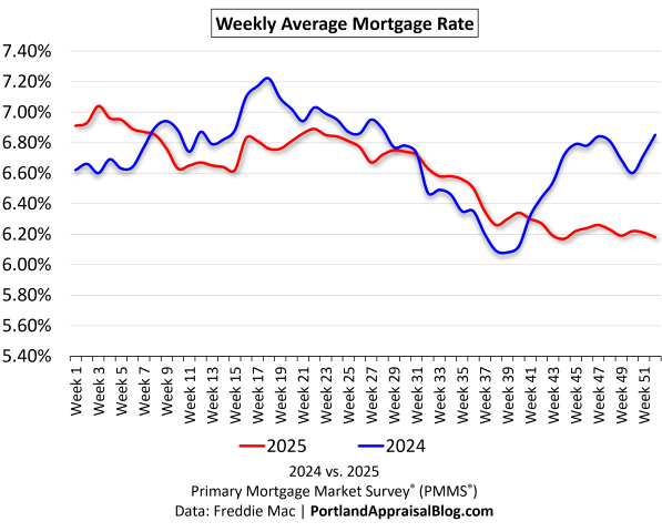
The market was not dominated by homes requiring substantially more income than the affordability threshold. Instead, many sales clustered immediately around it. As mortgage rates modestly improved during much of the 2025 selling season, required incomes fell enough to bring more homes into the affordability zone. Affordability was also buoyed by a rising HUD median family income for the Portland-Vancouver-Hillsboro MSA: $114,400 in 2024, rising to $124,100 by April 2025 and holding there through year-end.
PAB Insights is a Portland Appraisal Blog (PAB) series providing concise, data-driven answers to individual housing-market questions using transaction-level research, local market knowledge, and proprietary models, such as the Portland Appraisal Blog Affordability Index (PABAI).
Sources & Further Reading
All data presented in this PAB Insight is sourced directly from RMLS and has been subjected to our rigorous cleaning and validation process to ensure reliability for detached single-family residential analysis in the six-county Portland Region. The trends, comparisons, and commentary are the result of original appraisal expertise and independent analysis—not aggregated from secondary sources or news summaries.
PAB Insights: What Could Different Household Incomes Buy Among Troutdale’s Affordable Homes?: Portland Appraisal Blog
Coda
Thanks for reading—I hope you found a useful insight or an unexpected nugget along the way. If you enjoyed the post, please consider subscribing for future updates.
Are you an agent in Portland who wonders why appraisers always do “x”?
A homeowner with questions about appraiser methodology?
If so, feel free to reach out—I enjoy connecting with market participants across Portland and the surrounding counties, and am always happy to help where I can.
And if you’re in need of appraisal services in Troutdale or anywhere in the Portland Region, we’d be glad to assist.
About the Author — Abdur Abdul‑Malik, SRA, ASA
Abdur Abdul‑Malik is the founder, author, and publisher of the Portland Appraisal Blog, where he produces original regional and neighborhood‑level housing analytics for the Portland Region. He is a certified residential appraiser serving Oregon and Washington, drawing on RMLS transaction data, public records, and custom segmentation models he has built.
He developed the Portland Appraisal Blog Affordability Index (PABAI), a payment‑based affordability metric built from actual RMLS sales. PABAI incorporates weekly updates based on the prevailing 30‑year fixed mortgage rate, providing a locally grounded measure of housing affordability across the region.
Troutdale’s 2025 housing market generated more than $64 million in residential sales, with detached homes accounting for over 93% of all transactions. Affordability rose sharply; 35% of detached sales were affordable, up from 6%. This was due to softer prices and more favorable mortgage interest rates during peak selling season in 2025 compared with 2024.
Troutdale’s “Gateway to the Gorge” arch welcomes visitors to the city’s historic downtown district near the western entrance to the Columbia River Gorge. Photo: Abdur Abdul-Malik, Portland Appraisal Blog
About This Snapshot
This snapshot summarizes residential sales occurring within the official City of Troutdale limits during calendar year 2025 (with some comparisons to calendar year 2024). Included property types are detached homes, attached homes, condominiums, and manufactured homes on owned land. Data are sourced from RMLS and have undergone our standard cleaning and validation process. Manufactured homes located in leased-space parks are not included. For additional information regarding data cleaning procedures and common MLS data challenges, see the dedicated page: RMLS Data Accuracy Challenges.
Tables in this snapshot cover important metrics such as:
Sales price to original list price: SP/OLP
Price per square foot (total square footage): PPSF (TSF)
Cumulative days on market: CDOM
Average lot size in acres: ac
Market Overview
Located in eastern Multnomah County, Troutdale is a community in the Portland Region best known as the “Gateway to the Gorge.” Situated near the western entrance to the Columbia River Gorge, the city offers convenient access to outdoor recreation while remaining connected to the broader Portland metropolitan area.
Citywide Residential Market Snapshot
The following table summarizes residential sales occurring within Troutdale city limits during calendar year 2025. Included property types are detached homes, attached homes, condominiums, and manufactured homes on owned land. Together, these four segments provide a high-level overview of Troutdale’s owner-occupied residential market.
Category
Detached
Attached
Condo
Manuf.
Total Dollar Volume
$60,926,158
$2,652,800
$665,000
$0
Average Price
$495,335
$378,971
$332,500
—
Average PPSF (Total SF)
$302.51
$250.99
$226.84
—
Average Total SF
1,706
1,530
1,467
—
Average Lot Size (ac)
0.2160
0.0614
N/A
—
Average Age (Yrs)
37.38
17.00
21.50
—
Average CDOM
42.25
92.14
73.50
—
Total # of Sales
123
7
2
0
% of Market
93.18%
5.30%
1.52%
0.00%
Highest Sale
$840,000
$440,000
$350,000
—
Lowest Sale
$360,000
$332,800
$315,000
—
# Affordable
43
6
2
—
% Affordable
34.96%
85.71%
100.00%
—
January 2025 – December 2025 (132 total residential sales). Data: RMLS | PortlandAppraisalBlog.com
Detached homes accounted for the overwhelming majority of residential sales activity in Troutdale during 2025. Total residential dollar volume across all tracked housing segments reached approximately $64.2 million, with detached homes representing more than 93% of all sales and nearly 95% of total dollar volume. Attached homes and condominiums represented a relatively small share of the market, while no manufactured homes on owned land sold during the year. The following sections examine each segment in greater detail.
Detached Homes
Detached homes represent the largest and most active residential housing segment in Troutdale. Because detached properties accounted for more than 9 out of 10 sales during 2025, this segment provides the clearest view of local market conditions.
Detached Homes Market Statistics
The following table compares detached-home sales activity occurring within Troutdale city limits during 2024 and 2025. Metrics include sales volume, pricing, property characteristics, marketing times, and affordability.
Category
2024
2025
Change
Total $ Volume
$57,199,850
$60,926,158
+6.51%
Average Price
$510,713
$495,335
-3.01%
Median Price
$501,500
$479,000
-4.49%
Avg SP/OLP
99.27%
98.09%
-1.19 pts
Avg PPSF (TSF)
$298.54
$302.51
+1.33%
Avg HOA Dues
$30.80
$44.72
+45.20%
Avg Total SF
1,768
1,706
-3.52%
Avg Lot Size (ac)
0.2160
0.2121
-1.77%
Avg Age (Yrs)
35.32
37.38
+5.83%
Avg CDOM
39.07
42.25
+8.14%
Total # of Sales
112
123
+9.82%
# of New Constr.
0
0
—
# Affordable
7
43
+36 homes
% Affordable
6.25%
34.96%
+28.71 pts
Note: The calculated average HOA dues is for sales reporting nonzero HOA dues (24 sales for 2024 & 35 sales for 2025). All other metrics use the full dataset for each year. Single-Family Detached Residential | 2024 & 2025 Data: RMLS | PortlandAppraisalBlog.com
Detached-home sales activity increased during 2025, with total sales rising from 112 to 123 and total dollar volume increasing 6.51% to approximately $60.9 million. Despite stronger sales activity, both average and median sale prices declined modestly, while average days on market increased just 3 days, from 39 to 42 days. Buyers also gained slightly more negotiating leverage, with the average sale-to-original-list-price ratio declining from 99.27% to 98.09%.
The typical detached home sold during 2025 was somewhat smaller and slightly older than in 2024, while average price per square foot increased modestly. No new detached-home construction sales were recorded in either year, reinforcing Troutdale’s role as a largely resale-driven housing market. HOA participation remained a minority characteristic of the detached market, though the share of detached-home sales reporting HOA dues increased from approximately 21% in 2024 to 29% in 2025.
Detached Homes Sales by Price Range
The following table summarizes detached-home sales occurring within Troutdale city limits during 2025 by price range. In addition to sales volume, the table highlights the typical size and age of homes sold within each price band.
Troutdale’s detached-home market was concentrated in the middle price ranges during 2025. More than 89% of detached-home sales occurred between $400,000 and $599,999, with the $400,000-$499,999 range alone accounting for 71 of 123 sales. As sale prices increased, average home size generally increased as well, from approximately 1,500 square feet in the $400,000-$499,999 range to more than 3,200 square feet in the $700,000+ ranges.
While most sales occurred in homes built during the 1980s and 1990s, the two highest-priced detached-home sales were very different properties. One involved a nearly four-acre mixed-use development site along the Sandy River with an older home contributing little to overall value, while the other was a large historic residence with more than 5,000 square feet of living area and an accessory dwelling unit. These sales illustrate how Troutdale’s highest-priced properties can derive value from factors such as land, development potential, size, and unique property characteristics rather than age alone.
Detached Homes Affordability
The following table summarizes detached-home affordability in Troutdale during 2024 and 2025 using PABAI. In addition to the number and percentage of affordable sales, the table reports the highest affordable sale, the average sale price of affordable homes, and the average household income required to purchase those homes under prevailing market conditions at the time of sale.
Category
2024
2025
Change
Affordable Sales
7
43
+36 homes
% Affordable
6.25%
34.96%
+28.71 pts
Highest Affordable Sale
$445,000
$474,900
+6.72%
Avg Price
$409,080
$431,612
+5.51%
Avg Required Income
$108,737
$114,232
+$5,494.37
Affordable sales are determined using the Portland Appraisal Blog Affordability Index (PABAI), which evaluates each detached-home sale using prevailing mortgage rates, household income assumptions, taxes, insurance, and financing costs at the time of sale.
Detached-home affordability improved substantially during 2025. The number of affordable detached-home sales increased from 7 to 43, while the share of affordable sales increased from 6.25% to 34.96% of the market. The highest affordable detached-home sale increased from $445,000 in 2024 to $474,900 in 2025.
As shown above, mortgage rates were generally higher throughout much of 2024 than 2025. Combined with modest declines in detached-home prices, lower financing costs expanded the number of homes meeting the affordability standard even though the highest affordable detached-home sale changed very little.
The average affordable detached home sold for $431,612 during 2025 and required an estimated household income of approximately $114,232. While affordability remained far from universal, Troutdale offered substantially more attainable detached-home ownership opportunities in 2025 than in the prior year.
Attached Homes
Attached homes represent a small but distinct segment of Troutdale’s housing market. While sales activity is limited compared with detached homes, attached housing can provide an ownership alternative for buyers seeking lower-maintenance living or a smaller land component.
Attached Homes Market Statistics
The following table compares attached-home sales activity occurring within Troutdale city limits during 2024 and 2025. Due to the limited number of sales, the results are best viewed as descriptive measures of market activity rather than indicators of broader market trends.
Category
2024
2025
Change
Total $ Volume
$2,662,500
$2,652,800
-0.36%
Average Price
$443,750
$378,971
-14.60%
Median Price
$420,000
$390,000
-7.14%
Avg SP/OLP
96.36%
88.63%
-8.03 pts
Avg PPSF (TSF)
$289.56
$250.99
-13.32%
Avg HOA Dues
$159.00
$224.25
+41.04%
Avg Total SF
1,528
1,530
+0.19%
Avg Lot Size (ac)
0.0350
0.0614
+75.51%
Avg Age (Yrs)
6.67
17.00
+155.00%
Avg CDOM
47.50
92.14
+93.98%
Total # of Sales
6
7
+16.67%
# of New Constr.
2
0
-100.00%
# Affordable
4
6
+ 2 homes
% Affordable
66.67%
85.71%
+19.04 pts
Note: The calculated average HOA dues is for sales reporting nonzero HOA dues (1 sale for 2024 & 4 sales for 2025). All other metrics use the full dataset for each year. Single-Family Attached Residential | 2024 & 2025 Data: RMLS | PortlandAppraisalBlog.com
Attached-home sales represented a small portion of Troutdale’s residential market in both years, with only seven sales recorded during 2025. Despite the limited number of transactions, attached homes consistently contributed approximately $2.65 million in annual residential dollar volume during both 2024 and 2025.
Pricing measures, including average sale price, price per square foot, and sale-to-list-price ratio, were all lower in 2025 than in 2024. Because the attached-home market consists of a very small number of transactions, year-to-year changes are often skewed by compositional differences among the sales.
Attached Homes Affordability
The following table summarizes attached-home affordability in Troutdale during 2024 and 2025 using PABAI.
Category
2024
2025
Change
Affordable Sales
4
6
+2 homes
% Affordable
66.67%
85.71%
+19.04 pts
Highest Affordable Sale
$420,000
$405,000
-3.57%
Avg Price
$406,250
$368,800
-9.22%
Avg Required Income
$111,482
$104,015
-$7,466.98
Affordable sales are determined using the Portland Appraisal Blog Affordability Index (PABAI), which evaluates each attached-home sale using prevailing mortgage rates, household income assumptions, taxes, insurance, and financing costs at the time of sale.
Attached homes remained one of Troutdale’s most affordable ownership options during both years analyzed. Six of seven attached-home sales met the PABAI affordability standard during 2025, compared with four of six sales during 2024. The average required household income fell from approximately $111,000 to $104,000; largely due to lower average sales prices in 2025 compared to the previous year.
Because the attached-home market consists of only a handful of transactions each year, affordability results should be interpreted cautiously. Nevertheless, the segment consistently provided ownership opportunities at lower price points than the detached-home market, with a large majority of sales meeting the affordability standard in both years.
Condominiums
Condominiums represent a very small segment of Troutdale’s residential market. Like attached homes, due to the limited number of sales, the results are best viewed as descriptive measures of market activity rather than indicators of broader market trends.
Condominium Housing Market Statistics
The following table compares condominium sales activity occurring within Troutdale city limits during 2024 and 2025.
Category
2024
2025
Change
Total $ Volume
$1,804,900
$665,000
-63.16%
Average Price
$360,980
$332,500
-7.89%
Median Price
$347,000
$332,500
-4.18%
Avg SP/OLP
95.68%
95.65%
-0.03 pts
Avg PPSF (TSF)
$223.12
$226.84
+1.67%
Avg HOA Dues
$357.60
$415.00
+16.05%
Avg Total SF
1,634
1,467
-10.20%
Avg Age (Yrs)
21.80
21.50
-1.38%
Avg CDOM
55.20
73.50
+33.15%
Total # of Sales
5
2
-60.00%
# of New Constr.
0
0
—
# Affordable
4
2
-2 homes
% Affordable
80.00%
100.00%
+20.00 pts
Note: All metrics use the full dataset for each year (including HOA dues). Condominium Residential | 2024 & 2025 Data: RMLS | PortlandAppraisalBlog.com
Condominium sales activity remained limited during both years, with only five sales recorded in 2024 and two sales recorded in 2025. While Troutdale contains several condominium communities, recent sales activity was concentrated in a small number of developments. Most of the condominium sales occurring during the period analyzed were located within the Edgefield Meadows community, a townhome-style condominium development.
Pricing remained relatively stable despite the limited number of transactions. Average price per square foot changed very little between years. All condominium sales reported HOA dues, with average monthly dues increasing from approximately $358 to $415. Because the condominium market consists of only a handful of transactions each year, changes in individual metrics strongly reflect the mix of unit sales.
Condominium Housing Affordability
The following table summarizes condominium affordability in Troutdale during 2024 and 2025 using PABAI.
Category
2024
2025
Change
Affordable Sales
4
2
-2 homes
% Affordable
80.00%
100.00%
+20.00 pts
Highest Affordable Sale
$394,000
$350,000
-11.17%
Avg Price
$346,225
$332,500
-3.96%
Avg Required Income
$106,279
$107,724
+$1,445.28
Affordable sales are determined using the Portland Appraisal Blog Affordability Index (PABAI), which evaluates each condominium sale using prevailing mortgage rates, household income assumptions, taxes, insurance, and financing costs at the time of sale.
Condominium affordability remained strong during both years analyzed. Four of five condominium sales met the PABAI affordability standard during 2024, while both condominium sales recorded during 2025 qualified as affordable. Average affordable sale prices remained in the mid-$300,000 range, while the average required household income remained relatively stable near $106,000 to $108,000.
Because condominium activity in Troutdale is limited, affordability results are heavily influenced by the specific units that sell during a given year. Nevertheless, the available data indicate that condominiums remained among the city’s more attainable ownership options during both years analyzed.
The City of Troutdale seal, featuring the community’s long-standing connection to the Columbia River and its identity as the “Gateway to the Gorge.” Photo: Abdur Abdul-Malik, Portland Appraisal Blog
Key Takeaways
Troutdale’s housing market is, for practical purposes, a detached-home market. Detached homes accounted for the overwhelming majority of residential sales activity during 2025 and remain the property type that most clearly defines local housing conditions.
The city’s housing stock is primarily composed of resale housing rather than new homes. No new construction detached-home sales were recorded during either 2024 or 2025. Among detached-home sales occurring during the two-year period, construction dates ranged from 1893 to 2022, with the average home built in 1989.
While attached homes and condominiums provide alternative ownership opportunities, both segments remain relatively small and generate limited annual transaction volume compared with detached housing. For buyers looking to take advantage of their comparatively lower prices, such units do not come on the market very often and may require patience.
For buyers seeking a balance between affordability, access to the Portland Region, and proximity to outdoor recreation, Troutdale remains a community worth considering. Located at the gateway to the Columbia River Gorge, the city offers a housing market that remains more attainable than many higher-priced areas within the metropolitan region.
Sources & Further Reading
All data presented in this annual snapshot is sourced directly from RMLS and has been subjected to a rigorous cleaning and validation process to ensure reliability for each single-family residential housing segment analysis. The trends, comparisons, and commentary are the result of original appraisal expertise and independent analysis—not aggregated from secondary sources or news summaries.
Thanks for reading—I hope you found a useful insight or an unexpected nugget along the way. If you enjoyed the post, please consider subscribing for future updates.
Are you an agent in Portland who wonders why appraisers always do “x”?
A homeowner with questions about appraiser methodology?
If so, feel free to reach out—I enjoy connecting with market participants across Portland and the surrounding counties, and am always happy to help where I can.
And if you’re in need of appraisal services in Troutdale or anywhere in the Portland Region, we’d be glad to assist.
About the Author — Abdur Abdul‑Malik, SRA, ASA
Abdur Abdul‑Malik is the founder, author, and publisher of the Portland Appraisal Blog, where he produces original regional and neighborhood‑level housing analytics for the Portland Region. He is a certified residential appraiser serving Oregon and Washington, drawing on RMLS transaction data, public records, and custom segmentation models he has built.
He developed the Portland Appraisal Blog Affordability Index (PABAI), a payment‑based affordability metric built from actual RMLS sales. PABAI incorporates weekly updates based on the prevailing 30‑year fixed mortgage rate, providing a locally grounded measure of housing affordability across the region.
Q1 2026 manufactured‑home sales rose to 60 regionwide (+11), with activity across 33 cities and every Oregon county in the Portland Region. Lots under 0.50 acres made up 38% of sales, while two 100+‑acre closings pushed the regional average lot size to nearly 8 acres.
The Portland White Stag Sign Photographer: Jimmy Woo Via Unsplash.com
Introduction
Manufactured‑home activity across the region showed a steady and broadly distributed performance in Q1 2026. The segment continued to span both rural acreage and metro‑area communities, reflecting its long‑standing role as one of the most geographically diverse housing types in the region. Sales appeared in every county, with contributions from dozens of cities, reinforcing the segment’s reach across a wide range of neighborhoods, lot sizes, and property types.
This quarter also highlighted the dual nature of manufactured‑home inventory. Smaller urban and suburban parcels formed the core of the market, while a handful of large rural properties shaped the upper end of pricing and acreage variation. The mix of these two profiles—compact metro lots and expansive rural acreage—remains one of the defining characteristics of the segment and continues to influence how manufactured homes behave in scatter plots, averages, medians, and quarterly comparisons.
Overall, Q1 2026 offered a clear view of a stable and widely distributed manufactured‑home market, with patterns that align closely with long‑term regional trends. The sections that follow explore these dynamics in more detail, including county‑level activity, city contributions, acreage distribution, and the visual patterns that emerge when price, square footage, and land size are viewed together.
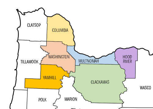
The Portland Region in this update comprises the six Oregon counties of Columbia, Clackamas, Hood River, Multnomah, Washington, and Yamhill. These counties form a contiguous housing ecosystem centered on Portland—Multnomah as the core home county, with the others tightly integrated through commuting patterns, economic ties, and shared market dynamics (e.g., Yamhill’s strong connection via Highway 99W and wine-country adjacency). Beyond Yamhill, the MLS system changes, further distinguishing this six-county area from broader geographic aggregations. For a detailed overview—including county profiles, population data, key value influencers, and why this definition differs from the official seven-county Portland–Vancouver–Hillsboro MSA—see the dedicated page: The Portland Region – Six-County Market Area Overview.
All data is sourced from RMLS and reflects open-market manufactured residential sales (excluding condominiums, attached homes, and site-built detached homes). SNL (“Sold Not Listed”) entries—off-market transactions entered retroactively—have been excluded to preserve consistency with true market activity.
All figures have undergone a rigorous data-cleaning process to address common RMLS accuracy challenges, including misclassifications (e.g. manufactured homes hiding in other categories such as detached), square footage/price typos, incomplete fields, status/date mismatches, and non-representative entries. For a detailed overview of these issues, their impact on market analysis, and how they are mitigated through automated flagging, cross-verification, and manual review, see the dedicated page: RMLS Data Accuracy Challenges.
It is important to note that this review focuses on manufactured homes permanently affixed to land that is also owned by the same party. This means we are excluding classic mobile-home parks where the owner of the mobile home must pay a lease/lot rental fee.
Portland Appraisal Blog Affordability Index (PABAI)
What PABAI Measures
The Portland Appraisal Blog Affordability Index (PABAI) is a model that estimates how home sale prices compare to what a median‑income household can qualify for under standard lending assumptions (HUD Portland-Vancouver-Hillsboro MSA median income, 20% down, and a 28% DTI for principal, interest, taxes, insurance, and HOA dues).
Unlike national affordability indices, PABAI is built from actual RMLS transactions rather than a single hypothetical price point. It computes an affordability ratio for every closed sale in the Portland Region during the analysis period using rates matched to the date of close, reported taxes, reported HOA dues, and an insurance estimate based on a percentage of the home’s value. The individual affordability ratios are then averaged to produce the reported PABAI value for that period.
For Q1 2026, this approach captures the actual mix of homes sold and the financing conditions present at the time those transactions occurred. Each housing segment—detached, attached, condos, and manufactured—is calculated separately, ensuring that segment‑specific dynamics are preserved rather than blended together. This provides a more detailed, locally grounded view of Portland‑area affordability and avoids the distortions that occur when fundamentally different housing types are combined into a single regional metric.
A PABAI of 100 means the market is exactly affordable at that income level (the Q1 2026 HUD median MSA income was $124,100 for a family of four). Values above 100 indicate excess qualifying capacity (more affordable), while values below 100 indicate a shortfall (strained affordability). Full methodology and the interpretation scale are available on the PABAI explainer page.
PABAI Range
Interpretation
120+
Strongly Affordable
100–119
Moderately Affordable
80–99
Strained
Below 80
Severely Constrained
Residential Housing Snapshot
Category
Detached
Attached
Condo
Manuf.
Total $ Volume
$2.2B
$161.0M
$199.0M
$32.4M
Avg Price
$659,197
$444,672
$389,438
$540,352
Avg PPSF (Total SF)
$316.21
$286.91
$325.55
$356.75
Avg Total SF
2,164
1,576
1,180
1,571
Avg Lot Size (ac)
0.655
0.066
N/A
7.959
Avg Age (Yrs)
46.03
15.09
32.03
29.10
Avg CDOM
80.22
80.59
119.62
118.25
# of Sales
3,349
362
511
60
% of Market
78.21%
8.45%
11.93%
1.40%
Highest Sale
$5,725,950
$1,175,000
$2,450,000
$2,400,000
Lowest Sale
$135,000
$249,000
$100,000
$199,700
Price Spread Ratio
42.41
4.72
24.50
12.02
PPSF Spread Ratio
30.93
4.08
11.91
13.29
Total SF Spread Ratio
23.46
4.14
12.24
3.52
Acreage Spread Ratio
5,182.19
19.54
—
1,559.53
Avg PABAI
85.45
110.38
122.83
118.04
Spread Ratio: A measure of how widely a variable ranges within the segment, calculated by dividing the largest value by the smallest. Q1 2026 (4,282 total residential sales). Data: RMLS | PortlandAppraisalBlog.com
The Portland Region’s residential market continues to operate as a tightly connected ecosystem, with each segment shaping and responding to the others in predictable ways. Detached homes remain the anchor segment—by far the largest in both sales count and dollar volume—and their scale sets the outer boundaries of regional pricing, land intensity, and buyer movement. With more than 3,300 sales and over $2.2 billion in closed volume this quarter, detached homes define the structural framework of the metro’s housing activity. Their wide spread ratios across price, PPSF, and size reflect a segment that spans everything from sub‑$150,000 fixers to multi‑million‑dollar estates. Detached homes also remain the least affordable segment, with a PABAI of 85.45, underscoring the gap between median incomes and the cost of entry into the region’s preferred housing type.
Attached homes sit directly beneath detached in the regional hierarchy and serve as the clearest alternative when detached becomes harder to access. They are the youngest segment in the metro—averaging just over 15 years old—and the most uniform, with tight spread ratios that signal a highly consistent, commodity‑like product. Their average price of $444,672 and moderate affordability (PABAI 110.38) position them as the region’s primary safety‑net for buyers priced out of detached homes. Attached homes represented 8.45% of all Q1 sales but played an outsized role in absorbing affordability‑sensitive demand, particularly in areas where detached prices have climbed beyond reach.
Condos remain the most affordable segment in the region, with a PABAI of 122.83 this quarter, but affordability alone does not translate into broad appeal. They are geographically concentrated—over two‑thirds of all condo sales occurred in Multnomah County—and their average age is more than double that of attached homes. HOA dues shape both buyer preferences and long‑term affordability, creating a segment where price ceilings are lower but carrying costs vary widely. Condos make up nearly 12% of all Q1 sales yet contribute less than 8% of total dollar volume, reflecting their structural role as an accessible option for some buyers but not a proportional driver of regional market activity.
Manufactured homes represent the smallest segment by far, with only 60 sales this quarter—just 1.40% of all regional activity. Their averages run high because many transactions include significant acreage: the typical manufactured home in Q1 2026 sat on nearly eight acres, a land profile unmatched by any other segment. This land intensity is the defining feature of manufactured homes and explains why their average price ($540,352) exceeds condos and attached homes despite similar dwelling sizes. Manufactured homes share several surface‑level similarities with condos—age, CDOM, affordability—but diverge sharply in how they trade: manufactured homes trade on land, while condos trade on dues. With such a small sample size, outliers exert more influence on segment averages than in any other category, and this sensitivity is a key consideration when interpreting manufactured‑home metrics.
Across the ecosystem, three of the four segments cluster in the low–mid $300s PPSF, underscoring that structure cost is relatively consistent across the metro. It is land, size, dues, and buyer preferences that create the separation between segments. Detached homes show the widest internal variation, attached homes the tightest, condos a bimodal profile shaped by older stock and boutique new construction, and manufactured homes a land‑driven spread that reflects acreage more than dwelling characteristics. This snapshot frames the broader regional context and sets the stage for the manufactured‑home‑specific analysis that follows.
Portland Region Q1 2026 Overview
Overall Regional Trends
The table below summarizes key metrics for manufactured homes residential sales in the Portland Region (Clackamas, Columbia, Hood River, Multnomah, Washington, and Yamhill counties) for Q1 2026 compared with Q1 2025.
Category
Q1 2025
Q1 2026
Change
Total $ Volume
$21,744,192
$32,421,110
+49.10%
Average Price
$443,759
$540,352
+21.77%
Median Price
$404,000
$432,450
+7.04%
Avg SP/OLP
95.06%
91.69%
-3.37 pts
Avg PPSF (TSF)
$301.16
$356.75
+18.46%
Avg HOA Dues
$106.33
$30.60
-71.22%
Avg Total SF
1,542
1,571
+1.88%
Avg Lot Size (ac)
3.55
7.96
+124.49%
Avg Age (Yrs)
30.92
29.10
-5.88%
Avg CDOM
78.35
118.25
+50.93%
Total # of Sales
49
60
+22.45%
# of New Constr.
1
2
+100.00%
# of REOs
0
2
—
# of Short Sales
0
3
—
Average PABAI
119.49
118.04
-1.45 pts
# Affordable
30
37
+7 homes
% Affordable
61.22%
61.67%
+0.45 pts
Note: The calculated average HOA dues is for sales reporting nonzero HOA dues (3 sales for Q1 2025 & 5 sales for Q1 2026). All other metrics use the full dataset for each quarter. Single-Family Manufactured Residential | Q1 2025 & Q1 2026 Data: RMLS | PortlandAppraisalBlog.com
Key Observations From the Aggregate Data
The Portland Region’s manufactured‑home market saw a meaningful increase in activity this quarter, with total dollar volume rising from $21.7 million in Q1 2025 to $32.4 million in Q1 2026. Sales count increased from 49 to 60, a sizable percentage gain but one that should be interpreted cautiously given the segment’s small size. Manufactured homes remain a low‑volume, land‑driven category, and even modest shifts in participation can produce large percentage changes. What stands out more than the increase in sales is the mix of properties that sold: Q1 2026 included several large‑acreage transactions that reshaped the segment’s averages and influenced many of the metrics in the regional overview table.
Average price rose sharply this quarter, increasing 21.77% year‑over‑year, but median price moved only 7.04%. This divergence is a classic mix effect. A handful of high‑acreage, high‑dollar properties pulled the average upward, while the median remained anchored to the typical manufactured home. The acreage distribution illustrates this clearly. The lowest‑acreage properties in both quarters were identical at 0.069 acres, but the upper end of the market expanded dramatically: the largest Q1 2025 sale sat on 34.18 acres, while Q1 2026 included a 107.37‑acre transaction. Median acreage nearly doubled from 0.92 to 1.77 acres, and average acreage more than doubled from 3.55 to 7.96 acres. Total square footage and age, by contrast, remained remarkably stable. The typical manufactured home in Q1 2026 was only 29 years old and just 29 square feetlarger than last year’s average. This stability reinforces the central dynamic of the segment: land is the wildcard variable, and acreage—not dwelling characteristics—drives most of the movement in price, CDOM, and SP/OLP.
Affordability also reflected the quarter’s mix. Despite improved mortgage rates, PABAI barely moved, slipping from 119.49 to 118.04. This stability is expected when the segment’s composition shifts toward larger, more expensive acreage properties. Even so, the number of affordable manufactured homes increased from 30 to 37, a meaningful gain for buyers seeking land‑included options within reach of median incomes. Manufactured homes remain one of the region’s more affordable ownership pathways, particularly for households seeking rural settings or acreage‑based utility.
SP/OLP declined from 95.06% to 91.69%, but this is not a market signal so much as a mix signal. High‑dollar manufactured homes—particularly those in the $1 million to $2 million range—often begin with ambitious list prices and require reductions before finding a qualified buyer. These properties also take longer to sell, contributing to the rise in CDOM from 78 to 118 days. As with SP/OLP, the increase in CDOM reflects the presence of large‑acreage, high‑price listings rather than a broad shift in buyer behavior or market conditions.
Taken together, the regional overview shows a manufactured‑home segment shaped primarily by land intensity and the presence of several large rural transactions. The underlying dwelling characteristics remained stable, affordability held steady, and the segment continued to operate as a small but meaningful part of the Portland Region’s housing ecosystem. This factual context sets the stage for the visual analysis that follows, where the scatter and bubble plots help illustrate how acreage influenced pricing and time on market in Q1 2026.
Portland Region Scatter Plots
To visualize the distribution of individual manufactured homes sales prices across Q1 2026, the following scatter plots show sales price against date of sale:
The scatter plot for Q1 2026 manufactured‑home sales shows a stable mid‑market band with a small number of large rural outliers that shaped the quarter’s averages. Nearly half of all sales this quarter—43.33%—closed between $300,000 and just under $500,000, forming the core of the market and creating the dense central cluster visible in the plot. Roughly 60% of the segment remained under $500,000, and 85% closed under $700,000, reinforcing the consistency of the mid‑range and the affordability profile that manufactured homes typically provide.
Above this central band, the scatter shows several high‑dollar outliers that influenced the quarter’s average price. Two sales exceeded $2 million, and another closed above $1.1 million. These properties sit well above the main cluster and visually demonstrate how a small number of large rural transactions can pull the average upward even when the median moves only modestly. Manufactured homes are uniquely sensitive to these outliers because the segment is small and land‑driven; a single high‑acreage sale can reshape the upper end of the scatter without altering the underlying structure of the mid‑market.
The timeline also reflects the segment’s naturally sporadic cadence. With only 60 sales this quarter, gaps between closings are expected and do not indicate any underlying shift in buyer behavior or market conditions. Manufactured homes trade infrequently, and their distribution across the quarter is shaped more by listing availability and rural transaction timing than by any broader trend.
Overall, the scatter plot illustrates a manufactured‑home market defined by a predictable mid‑market core and a small number of acreage‑driven outliers. The visual distribution aligns with the broader regional trends discussed earlier and provides a clear, factual foundation for the acreage‑based bubble analysis that follows.
To visualize three important variables at one, the following scatter plot shows sales price versus total square footage with each dot sized by acreage (lot size):
One of the most notable features of the plot is the presence of two very large bubbles near the top of the price range. These represent the highest‑dollar sales of the quarter, both closing above $2 million and both situated on exceptionally large lots—more than 100 acres each. Their size and position make clear how acreage drives the upper end of manufactured‑home pricing. The segment posted a land ratio of 1,559.53 this quarter, meaning the largest lot was nearly 1,560 times larger than the smallest lot. This underscores how dominant land value is within this category.
At the other end of the spectrum, many very small bubbles appear throughout the mid‑market band. 38.33% of all Q1 sales closed on lots under 0.50 acres, including properties located within the City of Portland and other urban or suburban settings. By the time the acreage reaches 1.50 acres, more than half the segment (51.67%) has already been accounted for. This wide spread—from compact city parcels to expansive rural acreage—is a defining characteristic of the segment and explains why manufactured homes show such large swings in average price and other metrics from quarter to quarter.
As the bubbles increase in size, a clear pattern emerges: larger bubbles naturally rise toward the upper end of the price range, while smaller bubbles cluster within the mid‑market. Manufactured homes with modest dwelling sizes but substantial land value tend to occupy the top of the scatter, while homes on smaller lots anchor the core of the market. The bubble plot makes this dynamic visually intuitive, showing how land—not square footage—is the primary driver of price variation within the segment.
Overall, this scatter plot reinforces the central theme of the manufactured‑home market in Q1 2026: a stable mid‑market core shaped by typical dwelling sizes, and a small number of large rural transactions that define the upper end of the price spectrum.
Counties & Top Cities Reporting Sales
The following table provides sales count for the region by county for Q1 2026 compared with Q1 2025:
Two observations stand out. First, Multnomah and Yamhill were the only counties that lost ground year‑over‑year, with modest declines of 3 and 4 homes respectively. Every other county posted gains, led by Clackamas (+8) and Washington (+7), both of which saw notable increases in manufactured‑home activity. Second, the region as a whole recorded a net gain of 11 manufactured‑home sales, reflecting a broader uptick in segment activity across Q1 2026.
A total of 33 cities reported at least one manufactured‑home sale in Q1 2026, reflecting the segment’s broad geographic reach across the region. To keep the table focused and readable, the summary below highlights cities with three or more sales during the quarter. These communities together accounted for 40.00% of all manufactured‑home activity, providing a clear view of where the segment was most concentrated.
Oregon City led the quarter with 6 sales, representing 10% of the entire manufactured‑home market. The remaining cities each contributed 3 sales, forming a balanced group of mid‑level contributors spread across Clackamas, Washington, Columbia, Hood River, and Yamhill counties.
The following map shows the geographic distribution of manufactured sales for Q1 2025 (blue pins) and Q1 2026 (red pins):
The pattern highlights the broad geographic reach of the segment, with activity appearing in every county and clustering along major corridors such as I‑84, Highway 26 and Highway 47. Rural areas continue to play a significant role in overall volume, but the map also shows a steady presence of manufactured‑home sales throughout the metro.
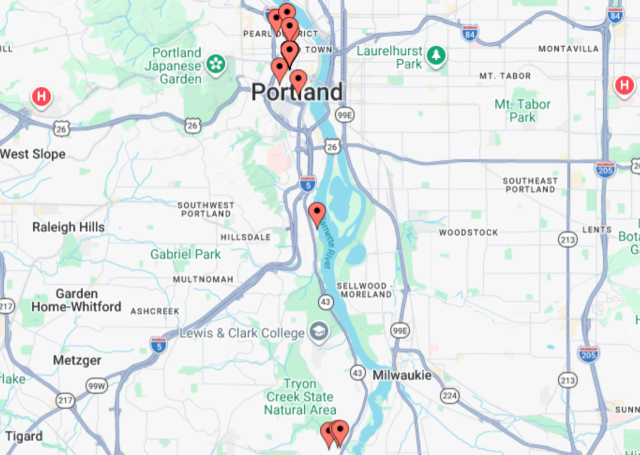
The following map shows the geographic distribution of manufactured sales centered around the City of Portland:
Unlike the regional map—where rural counties contribute many of the large‑acreage transactions—this metro‑focused view shows how consistently manufactured homes appear within the urban fabric of the region. Concentrations appear throughout Portland, Gresham, Sherwood, Beaverton, Newberg, and Oregon City, illustrating the steady presence of manufactured‑home activity within these city areas.
By isolating the Oregon portion of the metro, the map makes clear that manufactured homes are not limited to rural acreage or outlying counties. Many sales occur on smaller city and suburban parcels, aligning with earlier findings that 38.33% of Q1 2026 manufactured‑home sales closed on lots under 0.50 acres. The density of markers across the westside, eastside, and inner Portland neighborhoods reinforces the segment’s reach across a wide range of communities and lot sizes.
Closing Thoughts
Q1 2026 was a solid quarter for manufactured‑home activity across the region, marked by a meaningful year‑over‑year gain and a broad geographic footprint. The segment added 11 more sales than last year, with most counties posting increases and only Multnomah and Yamhill showing modest declines. The distribution of sales across 33 cities underscores how widely manufactured homes are represented throughout the region, from rural acreage to metro communities.
Acreage variation remained one of the defining characteristics of the segment. More than 38% of Q1 sales closed on lots under 0.50 acres, while two large rural transactions exceeded 100 acres, producing a spread ratio of nearly 1,560. This wide range continues to shape pricing behavior, with land value exerting a strong influence on the upper end of the market. The bubble‑scatter plot made this dynamic clear, showing how larger parcels naturally rise toward the top of the price spectrum while smaller urban and suburban lots anchor the mid‑market.
Taken together, Q1 2026 reflects a stable and geographically diverse manufactured‑home market—one shaped by a mix of small‑lot metro sales and a handful of large rural properties that continue to define the segment’s upper range. The majority of the movement in averages is simply due to the type of properties that closed this quarter.
What trends do you expect to see in Q2 2026? I’d love to hear your thoughts—feel free to reply here or reach out directly.
Sources & Further Reading
All data presented in this quarterly update is sourced directly from RMLS and has been subjected to our rigorous cleaning and validation process to ensure reliability for manufactured residential analysis in the six-county Portland Region. The trends, comparisons, and commentary are the result of original appraisal expertise and independent analysis—not aggregated from secondary sources or news summaries.
Thanks for reading—I hope you found a useful insight or an unexpected nugget along the way. If you enjoyed the post, please consider subscribing for future updates.
Are you an agent in Portland who wonders why appraisers always do “x”?
A homeowner with questions about appraiser methodology?
If so, feel free to reach out—I enjoy connecting with market participants across Portland and the surrounding counties, and am always happy to help where I can.
And if you’re in need of appraisal services in Portland or anywhere in the Portland Region, we’d be glad to assist.
About the Author — Abdur Abdul‑Malik, SRA, ASA
Abdur Abdul‑Malik is the founder, author, and publisher of the Portland Appraisal Blog, where he produces original regional and neighborhood‑level housing analytics for the Portland Region. He is a certified residential appraiser serving Oregon and Washington, drawing on RMLS transaction data, public records, and custom segmentation models he has built.
He developed the Portland Appraisal Blog Affordability Index (PABAI), a payment‑based affordability metric built from actual RMLS sales. PABAI incorporates weekly updates based on the prevailing 30‑year fixed mortgage rate, providing a locally grounded measure of housing affordability across the region.
The Q1 2026 Portland Region attached‑home update: median price $420k (‑5%), PPSF $287 (‑4%), sales +10%, dollar volume +4%. Affordability jumps to 69% (+41 pts) of the market. New construction +15%. County patterns, builder pivots, appraisal insights and more.
The Portland White Stag sign. Photo: Abdur Abdul-Malik, Portland Appraisal Blog
Introduction
The first quarter of 2026 was a study in contrasts across the Portland region’s attached‑home market. The three major counties—Multnomah, Washington, and Clackamas—continued to anchor the segment, each revealing its own distinct pattern of demand, pricing behavior, and builder activity. Together they formed the core of the regional story: softer prices, steady buyer engagement, and a noticeable shift in how builders are positioning new product. Beneath those broad themes, however, each county expressed the quarter differently, shaped by its inventory profile, geography, and development pipeline.
Washington County remained the region’s most uniform and predictable attached‑home market, with tight clustering in the mid‑price bands and a clear, data‑driven softening that still preserved strong absorption. Multnomah showed more variation, with affordability improving and pricing adjusting in a way that reflected both buyer sensitivity and the county’s diverse housing stock. Clackamas, by contrast, continued to operate at a higher price level, with a dense band of activity in the low‑$400s and a meaningful upper‑tier presence. Builders in Clackamas also made a notable pivot toward smaller new‑construction units—a strategic response to qualification thresholds that shaped the quarter’s pricing dynamics.
Outside the “Big Three,” the story was defined not by trends but by scale. Yamhill, Columbia, and Hood River each recorded only a handful of attached‑home sales, and their year‑over‑year changes reflected the volatility inherent in extremely small datasets. In these counties, a single closing can shift averages dramatically, and the absence of just a few transactions can reshape dollar volume.
Taken together, Q1 2026 shows a region adjusting to softer demand with realistic pricing, steady buyer participation, and builder strategies increasingly aligned with affordability constraints.
The Portland Region in this update comprises the six Oregon counties of Columbia, Clackamas, Hood River, Multnomah, Washington, and Yamhill. These counties form a contiguous housing ecosystem centered on Portland—Multnomah as the core home county, with the others tightly integrated through commuting patterns, economic ties, and shared market dynamics (e.g., Yamhill’s strong connection via Highway 99W and wine-country adjacency). Beyond Yamhill, the MLS system changes, further distinguishing this six-county area from broader geographic aggregations. For a detailed overview—including county profiles, population data, key value influencers, and why this definition differs from the official seven-county Portland–Vancouver–Hillsboro MSA—see the dedicated page: The Portland Region – Six-County Market Area Overview.
All data is sourced from RMLS and reflects open-market attached single-family residential sales. SNL (“Sold Not Listed”) entries—off-market transactions entered retroactively—have been excluded to preserve consistency with true market activity.
All figures have undergone a standard cleaning process to address common RMLS accuracy challenges, including misclassifications (such as condominiums listed as attached homes), square‑footage and price entry errors, incomplete fields, status/date mismatches, and other non‑representative entries. This post focuses exclusively on attached homes on owned land; while a condominium townhome and an attached townhome may appear similar, their ownership structures differ substantially. Condominiums are therefore carefully removed from this dataset. For a detailed overview of these issues, their impact on market analysis, and the mitigation steps used (automated flagging, cross‑verification, and manual review), see the dedicated page: RMLS Data Accuracy Challenges.
Portland Appraisal Blog Affordability Index (PABAI)
What PABAI Measures
The Portland Appraisal Blog Affordability Index (PABAI) is a model that estimates how home sale prices compare to what a median‑income household can qualify for under standard lending assumptions (HUD Portland‑Vancouver‑Hillsboro MSA median income, 20% down, and a 28% DTI for principal, interest, taxes, insurance, and HOA dues).
Unlike national affordability indices, PABAI is built from actual RMLS transactions rather than a single hypothetical price point. It computes an affordability ratio for every closed sale in the Portland Region during the analysis period using rates matched to the date of close, reported taxes, reported HOA dues, and an insurance estimate based on a percentage of the home’s value. The individual affordability ratios are then averaged to produce the reported PABAI value for that period. For Q1 2026, this approach captures the actual mix of homes sold and the financing conditions present at the time those transactions occurred. Each housing segment—detached, attached, condos, and manufactured—is calculated separately, ensuring that segment‑specific dynamics are preserved rather than blended together. This approach provides a more detailed, locally grounded view of Portland‑area affordability and avoids the distortions that occur when fundamentally different housing types are combined into a single regional metric.
A PABAI of 100 means the market is exactly affordable at that income level (the Q1 2026 HUD median MSA income was $124,100 for a family of four). Values above 100 indicate excess qualifying capacity (more affordable), while values below 100 indicate a shortfall (strained affordability). Full methodology and the interpretation scale are available on the PABAI explainer page.
PABAI Range
Interpretation
120+
Strongly Affordable
100–119
Moderately Affordable
80–99
Strained
Below 80
Severely Constrained
Note: While every sale produces an affordability ratio, the PABAI itself requires at least 20 sales to be statistically meaningful. Counties with fewer than 20 attached sales will report affordability counts and percentages, but not a PABAI.
Residential Housing Snapshot
Category
Detached
Attached
Condo
Manuf.
Total $ Volume
$2.2B
$161.0M
$199.0M
$32.4M
Avg Price
$659,197
$444,672
$389,438
$540,352
Avg PPSF (Total SF)
$316.21
$286.91
$325.55
$356.75
Avg Total SF
2,164
1,576
1,180
1,571
Avg Lot Size (ac)
0.655
0.066
N/A
7.959
Avg Age (Yrs)
46.03
15.09
32.03
29.10
Avg CDOM
80.22
80.59
119.62
118.25
# of Sales
3,349
362
511
60
% of Market
78.21%
8.45%
11.93%
1.40%
Highest Sale
$5,725,950
$1,175,000
$2,450,000
$2,400,000
Lowest Sale
$135,000
$249,000
$100,000
$199,700
Price Spread Ratio
42.41
4.72
24.50
12.02
PPSF Spread Ratio
30.93
4.08
11.91
13.29
Total SF Spread Ratio
23.46
4.14
12.24
3.52
Avg PABAI
85.45
110.38
122.83
118.04
Q1 2026 (4,282 total residential sales). Data: RMLS | PortlandAppraisalBlog.com
The four residential segments in the Portland Region continue to operate as a tightly connected ecosystem, each shaping and responding to the others in predictable ways. Detached homes remain the anchor segment—by far the largest in both sales count and dollar volume—and their scale sets the tone for regional pricing, land intensity, and buyer movement. With more than 3,300 sales and over $2.2 billion in closed volume this quarter, detached homes define the outer boundaries of what the market can deliver, from sub‑$150,000 fixers to multi‑million‑dollar estates. Their wide spread ratios across price, PPSF, and size reflect this internal diversity and underscore why detached remains the segment most buyers prefer even when affordability pushes them elsewhere.
Attached homes sit directly beneath detached in the regional hierarchy and serve as the clearest alternative when detached becomes harder to access. They are the youngest segment in the metro—averaging just over 15 years old—and the most uniform, with tight spread ratios that signal a highly consistent, commodity‑like product. Their average price of $444,672 and moderate affordability (PABAI 110.38) position them as the region’s primary safety‑net for buyers priced out of detached homes. The typical attached home is smaller, newer, and far more predictable in layout and utility than detached, and this consistency is a defining feature of the segment. In Q1 2026, attached homes represented 8.45% of all residential sales but played an outsized role in absorbing affordability‑sensitive demand.
Condos remain the most affordable segment in the region, with a PABAI of 122.83 this quarter, but affordability alone does not translate into broad appeal. They are also geographically concentrated: 67.71% of all condo sales occurred in Multnomah County, with most located in the City of Portland. This concentration reflects both historical development patterns and buyer preferences—condos are scarce or nonexistent in many suburban and rural areas where detached and attached homes dominate. Their average age is more than double that of attached homes, and HOA dues shape both buyer preferences and long‑term affordability. Condos make up nearly 12% of all Q1 sales yet contribute less than 8% of total dollar volume. Given the lower average price compared to all other segments, this gap is expected and reflects the structural role condos play in the ecosystem—an accessible option for some buyers, but not a proportional driver of regional dollar volume.
Manufactured homes represent the smallest segment by far, with only 60 sales this quarter. Their averages run high because many transactions include significant acreage—an average lot size of nearly eight acres—and with such a small sample, outliers exert more influence on segment averages than in any other category. Manufactured homes share several surface‑level similarities with condos (age, CDOM, affordability), but diverge sharply in how they trade: manufactured homes trade on land, while condos trade on dues.
Across the ecosystem, three of the four segments cluster in the low–mid $300s PPSF, underscoring that structure cost is relatively consistent across the metro. It is land, size, dues, and buyer preferences that create the separation between segments. Detached homes show the widest internal variation, attached homes the tightest, condos a bimodal profile shaped by older stock and boutique new construction, and manufactured homes a land‑driven spread that reflects acreage more than dwelling characteristics. This snapshot frames the broader regional context and sets the stage for the attached‑home‑specific analysis that follows.
Portland Region Q1 2026 Overview
Overall Regional Trends
The table below summarizes key metrics for attached homes residential sales in the Portland Region (Columbia, Clackamas, Hood River, Multnomah, Washington, and Yamhill counties) for Q1 2026 compared with Q1 2025.
Category
Q1 2025
Q1 2026
Change
Total $ Volume
$154,193,082
$160,971,196
+4.40%
Average Price
$470,101
$444,672
-5.41%
Median Price
$442,425
$420,250
-5.01%
Avg SP/OLP
97.30%
96.31%
-1.02%
Avg PPSF (TSF)
$297.52
$286.91
-3.56%
Avg HOA Dues
$243.36
$255.05
+4.81%
Median HOA Dues
$215.50
$233.00
+8.12%
Avg Lot Size (ac)
0.0621
0.0657
+5.71%
Avg Age (Yrs)
14.40
15.09
+4.85%
Avg CDOM
84.02
80.59
-4.07%
Avg Total SF
1,604
1,576
-1.76%
Total # of Sales
328
362
+10.37%
# of New Constr.
131
150
+14.50%
# of REOs
0
2
—
# of Short Sales
0
0
—
Average PABAI
93.43
110.38
+16.95 pts
# Affordable
118
250
+132 homes
% Affordable
35.98%
69.06%
+40.90 pts
Note: The calculated average HOA dues is for sales reporting nonzero HOA dues (260 sales for Q1 2025 & 279 sales for Q1 2026). All other metrics use the full dataset for each quarter. Single-Family Attached Residential | Q1 2025 & Q1 2026 Data: RMLS | PortlandAppraisalBlog.com
Key Observations From the Aggregate Data
The attached‑home segment softened meaningfully in Q1 2026, and the year‑over‑year comparison highlights a market adjusting to both price pressure and improved borrowing conditions. Average and median prices declined around five percent. This softness is not isolated—most counties saw similar declines—but Washington County’s dominance in attached‑home activity (51.38% of all regional sales) means its pricing trends exert the strongest pull on the regional averages. The ongoing impact of the Intel layoffs likely contributed to slightly faster market times, modestly lower prices, and a sharp improvement in affordability metrics.
Affordability is the standout story of the quarter. The segment flipped from strained to moderately affordable, with the PABAI jumping from 93.4 to 110.4. This is a substantial shift and reflects the combined effect of lower prices and better interest rates. The share of affordable attached homes surged from 35.98% to 69.06%, adding 132 more qualifying homes to the pool. This is not a compositional artifact; it is a direct response to improved lending conditions and softer pricing. When affordability improves, demand typically follows, and Q1 2026 delivered exactly that pattern.
Sales volume rose 10.37% year‑over‑year, and total dollar volume increased 4.40%. Importantly, the rise in dollar volume was driven by more sales, not higher prices. This distinction matters: it signals a market where buyers are re‑entering due to improved conditions rather than chasing rising values. The attached segment often acts as the pressure‑release valve for buyers priced out of detached homes, and this quarter’s data reinforces that role.
New construction played a meaningful part in the quarter’s dynamics. Closings increased from 131 to 150 (+14.50%), and Washington County accounted for roughly 60% of all new attached homes. This continues a multi‑year pattern in which Washington County favors new attached homes over new condos—a stark contrast to the condominium segment, which recorded zero new‑construction closings in Q1 2026. The slight increase in average age (14.40 → 15.09) despite more new construction indicates that the older resale stock still dominates the segment’s composition.
Market efficiency improved modestly. Cumulative days on market tightened from 84.02 to 80.59, and sellers yielded slightly more ground on pricing, with the average SP/OLP ratio dipping from 97.30% to 96.31%. These are small but meaningful signals of a market adjusting to softer pricing expectations. Distress remains negligible—only two REO sales and zero short sales—confirming that the segment’s softness is driven by normal market forces rather than financial stress.
Property characteristics remained stable. Square footage declined slightly (–1.76%), lot size held steady, and PPSF (based on total square footage) fell modestly (–3.56%). HOA dues increased, but only modestly (median +8.12%), far below the condominium segment’s 14% median jump. This stability reinforces that the segment’s year‑over‑year changes are driven primarily by pricing and interest‑rate dynamics rather than shifts in the underlying housing stock.
All six counties recorded attached‑home sales, though several had only a handful of closings. These counties will receive factual micro‑summaries later in the post, but the regional trends are overwhelmingly shaped by Multnomah, Washington, and Clackamas counties—with Washington County exerting the strongest influence due to its sheer volume.
Overall, Q1 2026 delivered a more affordable, more active, and slightly softer attached‑home market—one that responded predictably to improved rates and regional economic conditions. The segment’s role as the metro’s safety-net housing option is fully on display in this dataset.
Portland Region Scatter Plots
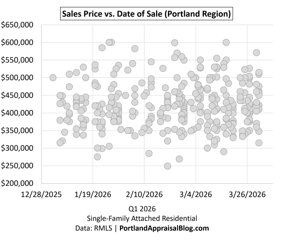
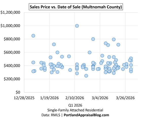
To visualize the distribution of individual attached homes sales prices across Q1 2026, the following scatter plots show sales price against date of sale:
The full‑quarter scatter plot provides a clear visual of how attached‑home prices distributed across Q1 2026. Even with normal day‑to‑day variation, the segment shows a remarkably tight mid‑market band: more than 70% of all attached sales closed between $350,000 and $499,999, and over 31% clustered specifically in the $400,000–$449,999 range. This concentration is exactly what the spread‑ratio metrics signal—attached homes are the metro’s most uniform, commodity‑like segment, with predictable layouts, consistent utility, and limited variation in size.
The scatter also shows a modest number of lower‑priced sales, but they are rare. Only eight sales closed below $300,000, and just one sale fell below $250,000. This scarcity reinforces the segment’s role in the ecosystem: attached homes are more affordable than detached, but they are not an entry‑level segment in the same way condos can be. Buyers seeking sub‑$300,000 opportunities generally must look to condominiums or manufactured homes.
At the upper end, the scatter includes a small number of premium attached homes, with roughly a dozen sales above $700,000 and three sales at or above $950,000. These outliers demonstrate that the segment can support higher‑end product in select neighborhoods, but they are too infrequent to influence regional averages or affordability metrics.
Activity is evenly distributed across the quarter, with no visible surges or drop‑offs. This aligns with the sales‑count data: closings increased year‑over‑year, driven by improved affordability and a notable rise in new‑construction deliveries. The scatter shows no abrupt price spikes or collapses—just a steady, slightly softer price environment consistent with the five‑percent decline in average and median values.
Overall, the full scatter plot reinforces the defining characteristics of the attached‑home segment: stable demand, tight pricing distribution, and a mid‑market profile that anchors the region’s affordability landscape.
Zooming in on sales priced at $600,000 or less, we have:
Note: The y-axis starts at $200,000 to allow better examination of the scatter plot.
The zoomed‑in scatter plot sharpens what the full‑scale view already suggested: attached‑home prices in Q1 2026 were tightly concentrated in the mid‑market band. With the vertical axis capped at $650,000, the plot highlights the segment’s core range—roughly $300,000 to $550,000—where nearly 80% of all sales occurred. The clustering is dense, consistent, and evenly distributed across the quarter, reinforcing the segment’s commodity‑like profile and the stability of demand throughout Q1.
The zoomed view also makes the lower‑priced portion of the market easier to see. Only a handful of sales fell below $300,000, and just one dipped below $250,000. This scarcity underscores that attached homes are not the region’s entry‑level segment; buyers seeking sub‑$300,000 opportunities overwhelmingly turn to condos or manufactured homes instead.
At the upper end, the zoomed plot shows a small number of sales pushing into the $600,000–$650,000 range. These are the same premium outliers visible in the full scatter, but the zoomed view makes clear how infrequent they are relative to the segment’s core. They represent neighborhood‑specific product rather than a broader trend.
Overall, the zoomed‑in scatter confirms the defining characteristics of the attached‑home segment: a tight, predictable price distribution; steady activity across the quarter; and a mid‑market profile that aligns with the segment’s role as the region’s primary affordability bridge between condos and detached homes.
Sales Volume
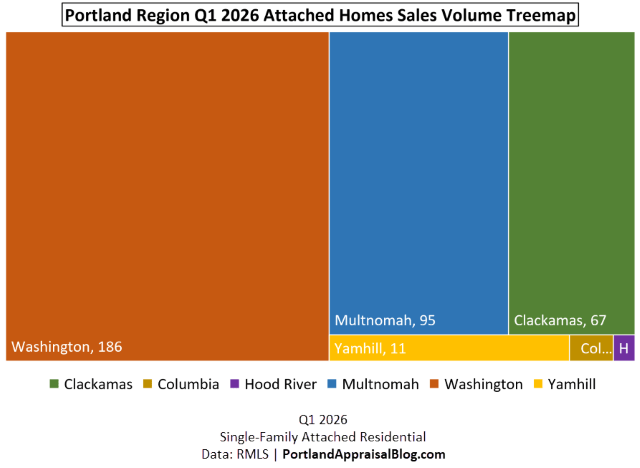
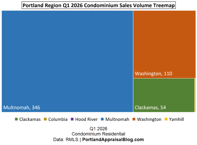
A treemap visualizing the distribution of attached homes sales by county in Q1 2026 clearly illustrates the market’s geographic concentration.
The treemap makes the geographic structure of the attached‑home market immediately clear: activity in Q1 2026 was overwhelmingly concentrated in the Big Three counties, with Washington County dominating the segment. More than half of all attached‑home closings occurred in Washington County alone, reflecting both its larger suburban housing base and its multi‑year preference for attached homes over condominiums. Multnomah and Clackamas counties round out the core, together contributing another 44% of all sales. In total, 96.13% of the region’s attached‑home activity came from the Big Three, underscoring how tightly the segment is anchored to the metro’s primary population and employment centers.
The remaining counties—Yamhill, Columbia, and Hood River—recorded only modest activity, with a combined 14 sales. These counties routinely produce small attached‑home counts due to their housing stock composition, development patterns, and buyer preferences. Their limited volume does not materially influence regional averages, but their participation confirms that attached homes are present, albeit sparsely, across the full six‑county region.
Washington County’s outsized share is especially important for interpreting regional trends. Because it accounts for 51.38% of all attached closings, its pricing, affordability, and new‑construction dynamics exert the strongest pull on the regional metrics discussed earlier. The treemap visually reinforces this influence: Washington County is not just the largest block—it is the structural center of the attached‑home market in Q1 2026.
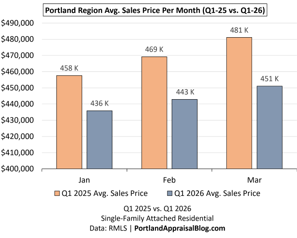
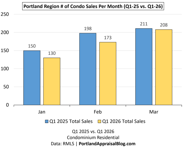
The bar chart below compares monthly sales volume across the three months of Q1 for 2025 and Q1 2026.
The month‑by‑month comparison highlights how attached‑home activity evolved across the quarter and why total sales ultimately finished higher than in Q1 2025. The pattern is uneven but intuitive: softer pricing and improved affordability brought more buyers back into the market, but the timing of that return varied by month.
January posted a modest increase, rising from 89 to 99 sales (+10). This aligns with the early‑quarter improvement in rates and the segment’s overall affordability shift. February, however, moved in the opposite direction, declining from 127 to 99 sales (–28).
March delivered the decisive shift. Sales jumped from 112 to 164 (+52), the strongest monthly gain of the quarter and the clearest signal of renewed buyer engagement. This surge is consistent with the broader Q1 narrative: affordability improved sharply, new‑construction closings increased, and the region’s core counties saw more buyers re‑enter the market.
While Washington County held nearly steady year‑over‑year, the overall increase in regional sales volume was driven by higher activity in Multnomah County, along with additional gains in Clackamas and Yamhill counties. These counties collectively tipped the scales, pushing the quarter to a 10.37% increase in total attached‑home sales.
Taken together, the monthly pattern shows a market responding predictably to improved conditions. Buyers returned gradually, then decisively, producing a strong finish to the quarter.
Sales Price
The bar chart below compares monthly average sales prices across the three months of Q1 for 2025 and Q1 2026.
Note: The y-axis starts at $400,000 to allow better examination of monthly differences.
Average sales prices declined across all three months of Q1 2026, and the pattern is both consistent and meaningful. January fell 4.75% year‑over‑year, February declined 5.60%, and March posted the steepest drop at 6.24%. While the magnitudes differ slightly, the direction is uniform: attached‑home prices were lower every month of the quarter compared to Q1 2025.
For buyers, this softening provided a genuine silver lining. Lower prices, paired with improved interest rates, helped push affordability sharply higher—one of the defining stories of the quarter. The attached segment flipped from strained to moderately affordable, and the monthly price declines played a direct role in that shift.
The softness was broad‑based. Every county except Hood River saw both average and median prices decline year‑over‑year. Hood River recorded only one attached sale, so its stability is not meaningful in a trend sense. The regional pattern reflects a tougher quarter for attached homes overall, and given that Washington County accounts for more than half of all attached closings, its slight year‑over‑year decline carries outsized influence. The ongoing Intel layoffs likely contributed to this pressure, adding a layer of economic uncertainty that nudged pricing expectations downward.
Even so, the segment remained active. Buyers responded predictably to improved affordability, and increased sales in Multnomah, Clackamas, and Yamhill counties helped offset Washington County’s slight decline. The result is a quarter where prices softened, affordability improved, and demand strengthened—an unusual but coherent combination that reflects the attached homes market’s multi-year trend of softening prices.
New Construction
The bar graph below shows monthly total attached homes sales in Q1 2026, with new construction volume nested within each bar to illustrate the portion of sales that were newly built.
The nested bar chart makes one point immediately clear: new construction is a defining feature of the attached‑home segment. Across Q1 2026, newly built homes accounted for 41.44% of all attached‑home closings, an unusually high share for any residential segment and fully consistent with attached homes having the lowest average age of the four major single-family housing categories.
The monthly pattern is also instructive. January and February delivered solid new‑construction activity, with 41 and 32 closings respectively—roughly one‑third to two‑fifths of all sales in each month. Then March surged. New‑construction closings jumped to 77, representing nearly 47% of all attached‑home sales that month.
Regionally, these figures underscore how central new construction is to the attached‑home ecosystem. The segment relies heavily on newly built supply to meet demand, and builders continue to deliver a substantial share of the product buyers ultimately purchase.
The bar graph below shows new construction sales broken out by county for Q1 2025 and Q1 2026.
The county‑level breakout highlights how unevenly new‑construction activity is distributed across the region and why the attached‑home segment continues to have the lowest average age of the four major housing categories.
Clackamas posted a modest gain, rising from 16 to 18 new‑construction closings (+12.50%). Washington County held essentially steady, dipping slightly from 91 to 90 (–1.10%). Multnomah, however, delivered the standout performance: new‑construction closings jumped from 24 to 40 (+66.67%), making it the fastest‑growing county in Q1 2026 for newly built attached homes. Yamhill added two new‑construction sales after recording none the prior year, while Columbia and Hood River remained at zero.
Even with Multnomah’s impressive growth, Washington County remains the structural center of new construction in the attached‑home segment. Its 90 closings represent 60% of all new‑construction activity—more than the remaining counties combined. This dominance is consistent with Washington County’s multi‑year pattern: it continues to favor new attached homes over new condos, and builders remain highly active in its suburban submarkets.
Regionally, the story is straightforward: new construction is not a supplemental source of inventory—it is a core driver of the attached‑home market. Q1 2026 reaffirmed that role with strong winter performance and a March surge, supported by notable gains in Multnomah and steady output from Washington County.
The table below shows new construction sales volume by dollar amount for Q1 2026 compared with Q1 2025.
The following double bar chart provides the above information at a glance.
New‑construction dollar volume rose modestly at the regional level in Q1 2026, increasing 3.66% year‑over‑year. But beneath that headline, the counties moved in very different directions—and understanding those differences is essential to interpreting the segment accurately.
Clackamas is the clearest example of a compositional reset rather than a pricing decline. Even though new‑construction sales increased from 16 to 18, total dollar volume fell sharply. The reason is straightforward: Q1 2025 included two exceptionally high‑end attached homes in Lake Oswego, each selling for more than $1.7M. Nothing in Q1 2026 exceeded the mid‑$500Ks. With those two luxury sales gone, the average price dropped significantly, but the median moved only modestly, reflecting a shift toward smaller, more affordable homes rather than a collapse in values.
Multnomah’s story is much simpler. New‑construction closings jumped from 24 to 40, and dollar volume rose accordingly. This is a clean volume‑driven increase, consistent with the county’s broader surge in attached‑home activity and its growing share of the region’s new‑construction market.
Washington County presents the opposite dynamic: sales were essentially unchanged, yet dollar volume declined. This signals genuine price softening, not a change in product mix. Builders conceded more on original list prices, average and median prices fell, price‑per‑square‑foot declined, and market times lengthened. Given Washington County’s outsized role in the attached‑home segment—and the economic backdrop created by the Intel layoffs—this softening resulted in builders netting roughly $3M fewer dollars year‑over‑year.
Taken together, these county‑level dynamics explain why regional dollar volume still managed a modest increase. Multnomah’s growth offset Washington County’s softening, and Clackamas’s compositional reset simply returned the county to its typical mid‑market profile. The result is a quarter where new construction remained a central driver of the attached‑home ecosystem, even as pricing pressures and product shifts varied sharply by county.
The following map shows the distribution of new construction sales.
The map of new‑construction closings reinforces a pattern that has been consistent for years: attached‑home new construction is overwhelmingly an urban and suburban phenomenon. The clusters concentrate along the westside and southside growth corridors—places like Hillsboro, Beaverton, Tigard, Sherwood, and Happy Valley—with smaller pockets extending into Gresham and the inner eastside.
What stands out is how tightly new construction hugs existing infrastructure, employment centers, and established development patterns. These aren’t rural builds or fringe‑market experiments; they’re infill projects, master‑planned communities, and suburban expansions in areas already primed for attached‑home demand. The distribution mirrors the segment’s identity: younger housing stock, smaller lots, and builder activity concentrated where land availability and zoning make attached homes feasible.
This spatial pattern also aligns with the county‑level dynamics discussed earlier. Washington County’s dominance is visible in the dense westside clusters, Multnomah’s growth shows up in the eastside and inner‑Portland pockets, and Clackamas’s contributions appear in the Happy Valley corridor.
Cumulative Days on Market
The bar chart below compares average cumulative days on market (CDOM) across the three months of Q1 for 2025 and Q1 2026.
The bar chart comparing average cumulative days on market across Q1 shows a clear and consistent pattern: the first two months of 2026 moved faster than the prior year, and those gains more than offset the slight lengthening in March.
January improved from 84 to 77 days (–8.32%), and February followed the same trajectory, dropping from 92 to 85 days (–7.62%). These early‑quarter improvements reflect stronger buyer engagement and quicker decision cycles at a time when mortgage rates were trending downward—moving from 6.16% to 5.98%. While rates aren’t the only factor influencing market tempo, this alignment likely contributed to the faster absorption we observed in January–February.
March, by contrast, saw average CDOM rise from 74 to 80 days (+7.21%). This coincided with a noticeable rate reversal, with mortgage rates climbing up 6.38% by month‑end. That shift likely introduced a bit of buyer hesitation and modestly slowed absorption. The increase wasn’t large enough to erase the momentum established earlier in the quarter, but it did slow the segment down.
Taken together, Q1 2026 still moved faster overall. The segment benefited from quicker early‑quarter absorption, and the modest recalibration in March reflects a market responding to short‑term rate movement rather than signaling a broader slowdown.
HOA Dues
While not all attached homes are located in an HOA with mandatory dues, they are a defining feature of the attached homes residential market:
Category
Q1 2025
Q1 2026
Change
# of HOA Sales
260
279
+19 homes
Total Sales
328
362
+34 homes
% of Market
79.27%
77.07%
-2.77 pts
HOA dues count are sales reporting nonzero HOA dues. Single-Family Attached Residential | Q1 2025 & Q1 2026 Data: RMLS | PortlandAppraisalBlog.com
The Q1 data shows just how central HOA‑based living is to the attached‑home segment. Out of 362 sales in Q1 2026, 279 reported nonzero HOA dues, meaning more than three‑quarters of all attached‑home closings occurred within dues‑bearing communities.
The increase in HOA‑dues sales—from 260 to 279—reinforces the stability of this pattern. Attached homes continue to be built, marketed, and purchased within communities where shared maintenance, common‑area amenities, and community standards shape both monthly payment profiles and long‑term ownership costs. HOA dues remain a defining financial component of the segment, influencing affordability calculations and distinguishing attached homes from their detached counterparts, which have much lower dues—averaging about $70 per month in the Big Three counties—and only 26% of sales occurring within HOAs.
In short, the attached‑home market continues to operate as a dues‑anchored ecosystem—HOA communities aren’t the exception; they’re the norm.
The bar chart below compares average monthly HOA dues (for reporting sales) for Q1 2025 and Q1 2026 broken out by county:
The county‑level comparison of average monthly HOA dues shows a mix of modest declines, one notable increase, and two counties that are omitted from the bar chart due to little or no attached‑home HOA activity in the period. Columbia had only a single dues‑bearing sale in Q1 2025 and none in Q1 2026, while Hood River’s dues figures are based on extremely limited sales and therefore aren’t included in the visual.
Clackamas, Multnomah, and Yamhill all posted year‑over‑year declines, while Washington County saw an increase from $238.66 to $259.44 (+8.71%). These shifts are meaningful, but interpretation requires attention to reporting behavior—especially in counties with active new‑construction pipelines.
Multnomah’s decline from $246.69 to $210.49 (–14.68%) should be read cautiously. The county saw a strong boost in new‑construction sales in Q1 2026, and it’s common for new‑construction listings to report zero HOA dues in MLS when dues haven’t been finalized at the time of listing. This can temporarily depress the average even when underlying dues are stable. Washington County, by contrast, had steady new‑construction activity year‑over‑year, making its increase more reliable and less affected by non‑reporting.
Yamhill’s decline is modest and should also be interpreted cautiously due to a small number of sales. Clackamas remains stable, with only a slight decrease.
Taken together, the county‑level data reinforces a familiar pattern: HOA dues vary across the region, but accurate interpretation requires accounting for reporting dynamics—especially in markets with active new construction.
Miscellaneous Statistics & Standout Transactions
Here are some of the most notable outliers and extremes from the 2026 Portland Region attached homes residential market—numbers that illustrate the full range of the data and the extremes buyers and appraisers encounter.
Lowest Sales Price: $249,000—This home is located in Wilkes Portland neighborhood. The unit is 1,114 sq. ft. and has two bedrooms and two bathrooms. Photos of this property are currently available online.
Highest Sales Price: $1,175,000—This home is located in Hood River, Oregon. The unit is 1,819 sq. ft. and has three bedrooms and three bathrooms. This property also has the highest price per square foot for the quarter ($645.95). Photos of this property are currently available online.
Lowest Price Per Square Foot: $158.13—This home is located in Lake Oswego, Oregon. The unit is 1,992 sq. ft., has three bedrooms and 2.1 bathrooms; it closed for $315,000. Photos of this property are currently available online.
Longest CDOM: 501 days—This home is located in the Northwest Heights Portland neighborhood. The unit is 1,431 sq. ft. and has two bedrooms and two bathrooms. Initially listed September 2024 for $450,000, it finally closed for $350,000 in late-February 2026. Photos of this property are currently available online.
Smallest Attached Home: 794 sq. ft.—This attached home is located in Newberg, Oregon. The one-bedroom, one-bathroom home is located in the 55+ community of Crestview Manor. Photos of this property are currently available online.
Largest Attached Home: 3,284 sq. ft.—The largest townhome of the quarter is located in West Linn, Oregon. The home has four bedrooms and 3.1 bathrooms. The unit closed for $897,500. Photos of this property are currently available online.
Highest Monthly HOA Dues: $793.00—This home is located in Lake Oswego, Oregon. The unit closed for $455,000 and is 1,314 sq. ft and has two bedrooms and two bathrooms. The HOA dues include a community pool, recreation facility as well as coverage of water, sewer, and exterior maintenance. Photos of this property are currently available online.
With the regional aggregate trends, graphs, monthly patterns, and notable outliers covered, the remainder of this update turns to a county-level breakdown. The following sections present year-over-year comparisons for each of the six counties in the Portland Region—Multnomah, Washington, Clackamas, Yamhill, Columbia, and Hood River. Each county snapshot includes key metrics, commentary on local drivers, and any segment-specific observations that help explain broader regional patterns.
Multnomah County Q1 2026 Stats
The table below summarizes key metrics for Multnomah County attached homes residential sales in Q1 2026 compared with Q1 2025.
Category
Q1 2025
Q1 2026
Change
Total $ Volume
$28,855,250
$40,935,465
+41.86%
Average Price
$450,863
$430,900
-4.43%
Median Price
$410,000
$395,000
-3.66%
Avg SP/OLP
96.50%
97.17%
+0.70%
Avg PPSF (TSF)
$319.62
$294.07
-8.00%
Avg HOA Dues
$246.69
$210.49
-14.68%
Median HOA Dues
$187.00
$178.00
-4.81%
Avg Lot Size (ac)
0.0566
0.0602
+6.41%
Avg Age (Yrs)
14.50
13.84
-4.54%
Avg CDOM
92.83
73.34
-21.00%
Avg Total SF
1,467
1,513
+3.12%
Total # of Sales
64
95
+48.44%
# of New Constr.
24
40
+66.67%
# of REOs
0
2
—
# of Short Sales
0
0
—
Average PABAI
98.92
119.88
+20.96 pts
# Affordable
36
72
+36 homes
% Affordable
56.25%
75.79%
+19.54 pts
Note: The calculated average HOA dues is for sales reporting nonzero HOA dues (31 sales for Q1 2025 & 41 sales for Q1 2026). All other metrics use the full dataset for each quarter. Single-Family Attached Residential | Q1 2025 & Q1 2026 Data: RMLS | PortlandAppraisalBlog.com
Multnomah County delivered a high‑volume quarter shaped overwhelmingly by new‑construction activity. Total dollar volume rose 41.86%, nearly proportional to the 48.44% increase in closed sales, confirming that the quarter’s strength came from more units selling, not higher prices.
Prices moved lower year‑over‑year despite slightly larger homes on slightly larger lots. Average price fell 4.43%, median price declined 3.66%, and average PPSF dropped 8.00%. This pattern reflects a clear compositional shift: new‑construction units averaged 1,350 square feet, compared with 1,631 square feet for resale units. Smaller homes enter the market at lower total prices even when their PPSF is strong, and Multnomah’s 40 new‑construction closings (up from 24) pulled the county’s pricing metrics downward.
Market tempo improved sharply. Average cumulative days on market fell from 92.83 to 73.34—a nearly 20‑day reduction. Builders tend to price new units to move, and the county’s elevated new‑construction share helped accelerate absorption. Sellers also gained a bit of ground relative to their initial list prices, with SP/OLP rising to 97.17%, indicating realistic initial pricing and responsive buyer demand.
HOA dues declined on both an average and median basis, but this drop is almost certainly illusory. New‑construction listings frequently report zero dues when HOA budgets are not finalized at the time of listing, and Multnomah’s surge in brand‑new inventory makes this reporting dynamic the most likely explanation for the decline.
Affordability expanded dramatically. The county’s PABAI rose to 119.88, and 75.79% of all sales qualified as affordable—more than three‑quarters of the market. This reflects both the influence of smaller, lower‑priced new‑construction units and the rate environment that supported stronger buyer access during the quarter. Builders are striving to meet the market where effective demand exists, and the Q1 delivery mix shows they were targeting price points buyers could actually reach.
Overall, Multnomah County’s Q1 2026 performance was defined by a large influx of smaller new‑construction homes, reshaping pricing, dues, affordability, and market tempo. The result was a fast‑moving, highly accessible quarter with strong buyer engagement and realistic seller pricing.
The following is a scatter plot of all Multnomah County attached homes sales in Q1 2026:
The scatter plot for Q1 2026 shows a market that is tightly concentrated in a very narrow price band. 76.84% of all Multnomah attached‑home sales closed between $300,000 and $500,000, which is an unusually compressed range compared with the detached‑home market. There is very little activity below $300,000 and only a small number of sales above $600,000, reinforcing just how centered this segment is around the mid‑market tiers.
The distribution is especially dense in the $350,000–$399,000 and $400,000–$449,000 brackets, which together account for more than half of all sales. The scatter reflects this visually: most points cluster in a tight vertical band, with only a few outliers pushing toward the upper end of the market.
The plot also shows a noticeable flurry of closings in the final stretch of March. At first glance, this might look like a demand‑side surge, but rates were climbing during that period—not the kind of environment that typically produces a sudden buyer rush. The timing instead reflects new‑construction deliveries closing out at quarter‑end, which becomes clear when isolating just the new‑construction sales.
When viewed alongside the main scatter, the new‑construction plot makes the pattern unmistakable: the late‑March cluster is a supply‑timed closing wave, not a rate‑driven spike in demand. Builders brought units online and pushed to finish the quarter strong, and those closings landed in a tight sequence at the end of March.
Together, the two scatters confirm a mid‑tier‑dominated market with minimal lower‑end activity, a thin upper tail, and a late‑quarter wave of new‑construction closings that helped lift overall volume.
The following map shows the distribution of new construction sales during Q1 2026:
The map of new‑construction sales shows a clear eastside concentration, and that pattern reflects the underlying development realities of Multnomah County. The eastside offers more flexible land availability, more accommodating zoning, and gentler topography, all of which support attached‑home projects at mid‑market price points. Builders can deliver units efficiently and at scale, and the result is the tight $300,000–$450,000 band seen in the new‑construction scatter.
The westside, by contrast, presents a very different development environment. Large portions of the westside are shaped by steep topography, constrained parcels, and higher‑priced neighborhoods where land costs and existing built form make attached‑home development less feasible. The economics simply don’t align with the mid‑tier price points where effective demand is strongest. As a result, new‑construction attached homes are far less common west of the Willamette, and the map reflects that imbalance clearly.
Together, the map and scatter plots show that new construction shaped not only the pricing and timing of Q1 2026, but also its spatial footprint—concentrated east of the river, aligned with the corridors where attached‑home development is most viable.
Washington County Q1 2026 Stats
The table below summarizes key metrics for Washington County attached homes residential sales in Q1 2026 compared with Q1 2025.
Category
Q1 2025
Q1 2026
Change
Total $ Volume
$86,314,512
$80,863,943
-6.31%
Average Price
$459,120
$434,752
-5.31%
Median Price
$444,177
$425,000
-4.32%
Avg SP/OLP
97.55%
95.70%
-1.89%
Avg PPSF (TSF)
$289.69
$277.49
-4.21%
Avg HOA Dues
$238.66
$259.44
+8.71%
Median HOA Dues
$232.00
$248.00
+6.90%
Avg Lot Size (ac)
0.0588
0.0623
+6.03%
Avg Age (Yrs)
13.84
13.98
+1.04%
Avg CDOM
76.13
86.90
+14.15%
Avg Total SF
1,609
1,588
-1.35%
Total # of Sales
188
186
-1.06%
# of New Constr.
91
90
-1.10%
# of REOs
0
0
—
# of Short Sales
0
0
—
Average PABAI
93.24
108.60
+15.36 pts
# Affordable
57
126
+69 homes
% Affordable
30.32%
67.74%
+37.42 pts
Note: The calculated average HOA dues is for sales reporting nonzero HOA dues (171 sales for Q1 2025 & 176 sales for Q1 2026). All other metrics use the full dataset for each quarter. Single-Family Attached Residential | Q1 2025 & Q1 2026 Data: RMLS | PortlandAppraisalBlog.com
Washington County’s attached‑home market softened in Q1 2026, and the declines are genuine. Withtotal sales down by only two homes and new‑construction volume essentially unchanged (91 → 90), the year‑over‑year comparison reflects real demand‑side cooling rather than a shift in unit mix. Average price, median price, SP/OLP, and PPSF all moved lower, while CDOM rose by about ten days—a pattern consistent with buyers becoming more cautious. The ongoing fallout from the Intel layoffs likely contributed to this softer environment, especially in the resale segment.
Despite only two fewer sales, sellers took in $5.45 million less this quarter compared to last year. That’s a meaningful drop in total dollar volume, and it underscores how broad the softening was: lower prices, lower PPSF, and slightly weaker negotiation outcomes all combined to pull revenue down.
Affordability, however, surged. More than two thirds of the market (67.74%) qualified as affordable under the PABAI framework, up from just 30.32% a year earlier. PABAI jumped by 37.42 points, reflecting how rate movements and softer pricing intersected to dramatically expand buyer qualification. And because new‑construction volume was nearly identical year over year, the usual issue of under‑reported HOA dues is effectively a wash—meaning the affordability trend is directionally reliable for Washington County, even though new‑construction dues remain understated in RMLS.
A side‑by‑side look at new construction versus resale in Q1 2026 shows a market that is almost perfectly split by both dollar volume and number of sales. New homes delivered slightly more square footage and larger lots, but the median price difference between new ($449,945) and resale ($410,500) was only about $40,000, indicating that Washington County does not impose a large premium for new attached homes.
Overall, Washington County’s attached‑home segment in Q1 2026 reflects a stable mix, softer demand, expanded affordability, and a nearly even split between new and resale activity. The declines are real, the affordability gains are meaningful, and the market’s performance is best understood as a demand‑side cooling rather than a structural or compositional shift.
The following is a scatter plot of all Washington County sales in Q1 2026:
The scatter plot shows a market operating within an exceptionally tight price band. Nearly the entire quarter’s activity falls between $300,000 and $500,000, and more than half the market (54.84%) is concentrated in the $350,000–$449,999 range. This mid‑tier clustering is the defining feature of Washington County’s attached‑home segment in Q1 2026, and the scatter makes it visually unmistakable: a dense horizontal band with very few outliers above $550,000 and almost nothing below $300,000.
There is a modest uptick in closings during March, reflecting two overlapping dynamics. First, Washington County saw a slight increase in new‑construction closings toward the end of the quarter, which naturally produces a small late‑March cluster. Second, the attached‑home market typically warms as spring approaches, and the scatter shows that familiar seasonal lift. Even so, the March activity remains firmly within the same mid‑tier band, reinforcing how stable and price‑disciplined the segment was throughout Q1.
Overall, the scatter confirms a highly concentrated mid‑market, minimal lower‑end activity, and only a thin upper tail. Washington County’s attached‑home market in Q1 2026 operated within one of the narrowest price distributions in the region, and the scatter plot visually mirrors the softness and affordability expansion seen in the county‑level metrics.
The following map shows the distribution of new construction sales during Q1 2026:
The new‑construction map for Washington County shows a development pattern that’s almost textbook for the westside: clusters of new attached‑home activity sitting right at the edges of cities, aligned with the urban growth boundary (UGB). The visual cue is unmistakable—the red markers concentrate precisely where the map transitions from urban coloration into green, signaling rural reserve, agricultural land, or forested areas. That boundary line is where Washington County’s attached‑home development has historically been most viable, and Q1 2026 continues that pattern.
Most of the new‑construction activity appears around Hillsboro, Aloha, Cornelius, and Forest Grove, with additional pockets near Bethany and South Beaverton. These are areas where land is still assemblable, topography is gentle, and zoning supports higher‑density formats. Builders gravitate to these UGB‑adjacent zones because they offer the combination of flat terrain, infrastructure access, and development‑friendly entitlements needed to deliver attached homes at mid‑tier price points.
What’s equally notable is where new construction isn’t happening. The interior of established neighborhoods—Cedar Hills, Sexton Mountain, Bull Mountain, central Beaverton—shows very few markers. These areas have higher land costs, fragmented parcels, and steeper topography in places, all of which make attached‑home development more difficult. The map’s pattern reflects that reality: new construction hugs the green edges rather than filling in the urban core.
Clackamas County Q1 2026 Stats
The table below summarizes key metrics for Clackamas County attached homes residential sales in Q1 2026 compared with Q1 2025.
Category
Q1 2025
Q1 2026
Change
Total $ Volume
$32,731,115
$33,201,588
+1.44%
Average Price
$536,576
$495,546
-7.65%
Median Price
$467,500
$440,000
-5.88%
Avg SP/OLP
97.43%
96.35%
-1.11%
Avg PPSF (TSF)
$299.00
$294.75
-1.42%
Avg HOA Dues
$286.20
$286.19
-0.00%
Median HOA Dues
$225.50
$243.00
+7.76%
Avg Lot Size (ac)
0.07
0.08
+6.16%
Avg Age (Yrs)
14.56
17.91
+23.03%
Avg CDOM
106.95
76.82
-28.17%
Avg Total SF
1,762
1,692
-3.98%
Total # of Sales
61
67
+9.84%
# of New Constr.
16
18
+12.50%
# of REOs
0
0
—
# of Short Sales
0
0
—
Average PABAI
84.89
97.72
+12.83 pts
# Affordable
14
39
+25 homes
% Affordable
22.95%
58.21%
+35.26 pts
Note: The calculated average HOA dues is for sales reporting nonzero HOA dues (50 sales for Q1 2025 & 56 sales for Q1 2026). All other metrics use the full dataset for each quarter. Single-Family Attached Residential | Q1 2025 & Q1 2026 Data: RMLS | PortlandAppraisalBlog.com
Clackamas County posted a mixed performance in Q1 2026, with rising sales activity but clear price erosion. Total sales increased nearly 10% year over year (61 → 67), yet total dollar volume rose only 1.44%, meaning sellers collectively earned just $470,473 more than last year. That gap between unit growth and revenue growth is the clearest sign of softening prices: average price fell 7.65%, median price declined 5.88%, and PPSF slipped modestly. Some of this decline reflects a shift toward smaller units—average total square footage dropped by nearly 4%—but the price reductions exceed what size alone would explain, indicating genuine market cooling.
Affordability expanded sharply, rising from 22.95% to 58.21%, yet Clackamas still remains the least affordable of the three major counties. Larger average square footage, higher HOA dues, and an older attached‑home stock all contribute to this structural reality. The average age of sold units jumped from 14.6 to 17.9 years, reinforcing that Clackamas has fewer new attached‑home projects and a more mature inventory profile compared with Multnomah and Washington counties.
One of the more notable improvements was in market efficiency: CDOM fell dramatically, dropping from 107 days to 77 days. Even with lower prices, homes sold significantly faster, suggesting sellers adjusted expectations and buyers responded to more realistic pricing. This is consistent with a market that is softening but still liquid.
A closer look at new construction versus resale in Q1 2026 shows that builders and resale sellers operated in distinctly different segments. New construction accounted for 18 sales, while resale represented 49, and the two cohorts diverged sharply in size. New homes averaged 1,572 sq. ft., compared with 1,736 sq. ft. for resale—a 164 sq. ft. difference that explains most of the pricing gap. Builders are clearly delivering smaller new units to keep average prices down—1,920 sq. ft. in Q1 2025 to 1,572 sq. ft. in Q1 2026—and when adjusting for square footage, the new‑construction premium essentially disappears. PPSF is nearly identical between the two groups, and a back‑of‑the‑envelope calculation shows that equal‑sized units would have nearly the same implied value.
Overall, Clackamas County’s attached‑home market in Q1 2026 reflects higher sales activity, lower prices, faster absorption, and a meaningful shift toward smaller new‑construction units. The county remains the least affordable of the Big Three, but the quarter shows a market adjusting efficiently to softer demand and delivering product that aligns with buyer qualification thresholds.
The following is a scatter plot of all Clackamas County sales in Q1 2026:
The scatter plot for Clackamas County shows a price distribution that is both tightly concentrated in the mid‑market and meaningfully stretched into the upper tiers, a pattern that distinguishes the county from both Multnomah and Washington. The densest portion of the quarter’s activity sits between $400,000 and $449,999, and when combined with the adjacent $450,000–$499,999 tier, these two ranges account for nearly three‑quarters of all sales. This narrow mid‑market band is the defining feature of Clackamas attached‑home pricing in Q1 2026.
What’s equally notable is what the scatter doesn’t show: almost no activity below $350,000. Only one sale fell into the 300–349K range, and nothing transacted below that. This absence of lower‑priced units is a structural characteristic of Clackamas County’s attached‑home stock—larger average square footage, higher HOA dues, and older inventory all push the market upward compared with the other major counties. The scatter makes this visually obvious: the lower end is essentially missing.
Above the mid‑market band, Clackamas shows a meaningful upper tail. Several sales closed between $600,000 and $1,000,000, including one above $950,000. This upper‑tier activity is far more pronounced than in Washington County, where attached‑home pricing is tightly uniform and rarely reaches these levels. In contrast, Clackamas supports a wider range of attached‑home formats and sizes, and the scatter reflects that diversity with a broader vertical spread.
Taken together, the scatter plot illustrates why Clackamas remains the least affordable of the Big Three counties. While all three counties struggle to produce units under $300,000, Multnomah’s densest band sits lower (350–399K), and Washington has substantial activity in the 300–399K range. Clackamas, by contrast, clusters higher and shows more upper‑tier sales, reinforcing the county’s structurally elevated pricing profile.
The following map shows the distribution of new construction sales during Q1 2026:
The new‑construction map for Clackamas County shows a pattern that’s immediately recognizable once you’ve looked at Multnomah and Washington: activity generally clusters right at or just inside the edges of major cities, where zoning, infrastructure, and parcel configuration make attached‑home development feasible. Every red marker sits in or near an incorporated area—Happy Valley, Milwaukie, Oregon City—and even the outlier in Molalla is still within the city’s built‑up footprint rather than in rural reserve or agricultural land. This is the same development logic we saw in Washington County, but expressed through Clackamas’ geography.
Yamhill County Q1 2026 Stats
The table below summarizes key metrics for Yamhill County attached homes residential sales in Q1 2026 compared with Q1 2025.
Category
Q1 2025
Q1 2026
Change
Total $ Volume
$1,996,000
$4,026,200
+101.71%
Average Price
$399,200
$366,018
-8.31%
Median Price
$400,000
$377,900
-5.53%
Avg SP/OLP
100.22%
97.45%
-2.77%
Avg PPSF (TSF)
$323.68
$311.36
-3.81%
Avg HOA Dues
$97.17
$87.92
-9.52%
Median HOA Dues
$65.00
$45.00
-30.77%
Avg Lot Size (ac)
0.09
0.09
-1.65%
Avg Age (Yrs)
25.60
24.91
-2.70%
Avg CDOM
23.20
76.91
+231.50%
Avg Total SF
1,262
1,201
-4.81%
Total # of Sales
5
11
+120.00%
# of New Constr.
0
2
—
# of REOs
0
0
—
# of Short Sales
0
0
—
# Affordable
4
11
+7 homes
% Affordable
80.00%
100.00%
+20.00 pts
Note: The calculated average HOA dues is for sales reporting nonzero HOA dues (4 sales for Q1 2025 & 5 sales for Q1 2026). All other metrics use the full dataset for each quarter. Single-Family Attached Residential | Q1 2025 & Q1 2026 Data: RMLS | PortlandAppraisalBlog.com
Yamhill County saw a sharp increase in attached‑home activity in Q1 2026, though the small sample size limits interpretation. Total sales rose from 5 to 11, a 120% increase, and total dollar volume more than doubled, netting sellers an additional $2.03M. With only a handful of transactions in each quarter, this jump reflects the addition of a few more closings rather than a structural shift in the market.
Two new‑construction units closed during the quarter, both from the same small infill project in Lafayette. This was the only new‑construction activity in the county for Q1 2026.
Overall, Yamhill County’s attached‑home market remains extremely low‑volume, and the quarter’s results reflect the sensitivity of small datasets to individual sales. The doubling of dollar volume and sales count is notable, but not indicative of a broader trend. The presence of two new units in Lafayette is the only structural change worth noting; otherwise, the quarter’s metrics should be interpreted cautiously due to limited activity.
The following is a scatter plot of all Yamhill County sales in Q1 2026:
Most activity is concentrated between $350,000 to under $450,000.
Columbia County Q1 2026 Stats
The table below summarizes key metrics for Columbia County attached homes residential sales in Q1 2026 compared with Q1 2025.
Category
Q1 2025
Q1 2026
Change
Total $ Volume
$2,811,205
$769,000
-72.65%
Average Price
$401,601
$384,500
-4.26%
Median Price
$405,000
$384,500
-5.06%
Avg SP/OLP
95.55%
98.81%
+3.41%
Avg PPSF (TSF)
$248.84
$246.68
-0.87%
Avg HOA Dues
$21.25
—
—
Median HOA Dues
$21.25
—
—
Avg Lot Size (ac)
0.08
0.08
+6.25%
Avg Age (Yrs)
19.86
27.00
+35.97%
Avg CDOM
45.86
13.00
-71.65%
Avg Total SF
1,633
1,560
-4.45%
Total # of Sales
7
2
-71.43%
# of New Constr.
0
0
—
# of REOs
0
0
—
# of Short Sales
0
0
—
# Affordable
6
2
-4 homes
% Affordable
85.71%
100.00%
+14.29 pts
Note: The calculated average HOA dues is for sales reporting nonzero HOA dues (2 sales for Q1 2025 & 0 sales for Q1 2026). All other metrics use the full dataset for each quarter. Single-Family Attached Residential | Q1 2025 & Q1 2026 Data: RMLS | PortlandAppraisalBlog.com
Columbia County had very limited attached‑home activity in Q1 2026, with only two sales recorded for the quarter. This represents a decline of five sales year‑over‑year, and total dollar volume fell accordingly—from $2.81M to $769,000, a reduction of $2.04M. With such a small dataset, these changes reflect the absence of a few transactions rather than any meaningful shift in market conditions. There were no new‑construction units this quarter.
Overall, Columbia County’s attached‑home market remains extremely low‑volume, and the quarter’s results should be interpreted cautiously. The decline in sales and dollar volume is notable, but not indicative of a structural change; it simply reflects the sensitivity of small datasets to individual transactions.
Hood River County Q1 2026 Stats
The table below summarizes key metrics for Hood River County attached homes residential sales in Q1 2026 compared with Q1 2025.
Category
Q1 2025
Q1 2026
Change
Total $ Volume
$1,485,000
$1,175,000
-20.88%
Average Price
$495,000
$1,175,000
+137.37%
Median Price
$460,000
$1,175,000
+155.43%
Avg SP/OLP
95.85%
106.82%
+11.44%
Avg PPSF (TSF)
$356.60
$645.95
+81.14%
Avg HOA Dues
$36.46
$401.91
+1002.48%
Median HOA Dues
$36.46
$401.91
+1002.48%
Avg Lot Size (ac)
0.0533
0.0300
-43.78%
Avg Age (Yrs)
12.67
21.00
+65.79%
Avg CDOM
114.00
25.00
-78.07%
Avg Total SF
1,501
1,819
+21.16%
Total # of Sales
3
1
-66.67%
# of New Constr.
0
0
—
# of REOs
0
0
—
# of Short Sales
0
0
—
# Affordable
1
0
-1 home
% Affordable
33.33%
0.00%
-33.33 pts
Note: The calculated average HOA dues is for sales reporting nonzero HOA dues (2 sales for Q1 2025 & 1 sale for Q1 2026). All other metrics use the full dataset for each quarter. Single-Family Attached Residential | Q1 2025 & Q1 2026 Data: RMLS | PortlandAppraisalBlog.com
Hood River County had only one attached‑home sale in Q1 2026, down from three the year before. With such a small dataset, year‑over‑year comparisons are not meaningful. Total dollar volume declined from $1.49M to $1.18M, a net difference of $310,000. There were no new‑construction units this quarter.
Overall, Hood River County’s attached‑home market remains extremely low‑volume, and the quarter’s results should be interpreted cautiously. The decline in sales and dollar volume is notable, but not indicative of a structural change; it simply reflects the sensitivity of small datasets to individual transactions.
Closing Thoughts
Q1 2026 showed a region adjusting through lower prices, slightly improved interest rates, and builder‑driven shifts in product size, all of which combined to make attached homes more accessible to buyers. With softer pricing, overall activity increased: regional sales rose 10%, and total dollar volume edged up 4.4%, signaling steady demand as buyers responded to more attainable price points.
Affordability was the standout change. The share of affordable attached‑home sales jumped from 20% to 61%, adding 155 more affordable units compared with last year. This improvement was driven primarily by lower prices, better mortgage rates, and a clear builder pivot toward smaller units in counties like Washington and Clackamas. New construction rose 14.5%, and much of that growth came from projects intentionally designed to meet buyer qualification thresholds.
The county distribution remained familiar: Washington County accounted for just over half of all attached‑home sales, Multnomah contributed about a quarter, and Clackamas nearly a fifth. The remaining counties—Yamhill, Columbia, and Hood River—continued to show extremely low volumes, where individual sales can shift averages dramatically and trend analysis is not meaningful.
Taken together, the quarter reflects a market that is re‑calibrating rather than contracting. Prices softened, affordability expanded, and builders adapted quickly to buyer needs.
What trends do you expect to see in Q2 2026? I’d love to hear your thoughts—feel free to reply here or reach out directly.
Sources & Further Reading
All data presented in this quarterly update is sourced directly from RMLS and has been subjected to a rigorous cleaning and validation process to ensure reliability for attached homes residential analysis in the six-county Portland Region. The trends, comparisons, and commentary are the result of original appraisal expertise and independent analysis—not aggregated from secondary sources or news summaries.
External Obsolescence in Hillsboro — Residential Market Response to Intel’s 2024–2025 Workforce Reductions: Portland Appraisal Blog
Coda
Thanks for reading—I hope you found a useful insight or an unexpected nugget along the way. If you enjoyed the post, please consider subscribing for future updates.
Are you an agent in Portland who wonders why appraisers always do “x”?
A homeowner with questions about appraiser methodology?
If so, feel free to reach out—I enjoy connecting with market participants across Portland and the surrounding counties, and am always happy to help where I can.
And if you’re in need of appraisal services in Portland or anywhere in the Portland Region, we’d be glad to assist.
About the Author — Abdur Abdul‑Malik, SRA, ASA
Abdur Abdul‑Malik is the founder, author, and publisher of the Portland Appraisal Blog, where he produces original regional and neighborhood‑level housing analytics for the Portland Region. He is a certified residential appraiser serving Oregon and Washington, drawing on RMLS transaction data, public records, and custom segmentation models he has built.
He developed the Portland Appraisal Blog Affordability Index (PABAI), a payment‑based affordability metric built from actual RMLS sales. PABAI incorporates weekly updates based on the prevailing 30‑year fixed mortgage rate, providing a locally grounded measure of housing affordability across the region.
Q1 2026 Portland Region condo update: average price $389k (+6.5%), median $325k (‑1.5%), sales 511 (‑8.6%), CDOM 119 days (+8%). Dollar volume dipped 2.6% as new construction fell sharply, yet still reached $199M. County trends diverged, and Ritz‑Carlton closings—after a year of no activity—kept the market from sliding further.
The City of Portland skyline with Mt. Hood in the distance. Via Canva Pro
The condo market entered 2026 on softer footing, with sales and dollar volume both slipping from last year’s pace. Activity was steady enough to keep the segment functional, but not strong enough to overcome the broader contraction. What complicated the picture was the renewed momentum at the Ritz‑Carlton Residences, which re‑emerged this quarter as a major force in the luxury segment. That revival reshaped the composition of what sold and kept the quarter from appearing weaker on the surface than the fundamentals alone would suggest.
The Ritz accounted for 60% of all $1M‑and‑up closings, and that concentration was enough to push average prices higher even as the rest of the market softened. Median prices, price‑per‑square‑foot, and total dollar volume all declined, reflecting a quieter underlying market. But the surge in luxury‑tower activity created a split narrative: the averages moved one way, the fundamentals another. It was a quarter defined less by broad price movement and more by what sold and where those sales occurred.
Affordability technically improved this quarter, and condos remain the most accessible segment for a median‑income household. But that improvement came from lower mortgage rates, not from dramatic changes within the condo market itself. Rising HOA dues continue to be a structural drag, and the segment’s geographic concentration limits its appeal. Many buyers still prefer detached homes with yards, and many prefer suburban or rural settings where condos are scarce or nonexistent. In that sense, condos remain affordable but not a panacea—an option that works well for some buyers, but not a broad solution to the region’s housing pressures.
The Portland Region in this update comprises the six Oregon counties of Columbia, Clackamas, Hood River, Multnomah, Washington, and Yamhill. These counties form a contiguous housing ecosystem centered on Portland—Multnomah as the core home county, with the others tightly integrated through commuting patterns, economic ties, and shared market dynamics (e.g., Yamhill’s strong connection via Highway 99W and wine-country adjacency). Beyond Yamhill, the MLS system changes, further distinguishing this six-county area from broader geographic aggregations. For a detailed overview—including county profiles, population data, key value influencers, and why this definition differs from the official seven-county Portland–Vancouver–Hillsboro MSA—see the dedicated page: The Portland Region – Six-County Market Area Overview.
All data is sourced from RMLS and reflects open-market condominium residential sales. SNL (“Sold Not Listed”) entries—off-market transactions entered retroactively—have been excluded to preserve consistency with true market activity.
Since condominium is an ownership type and not necessarily a description of style, a strict examination was made of all other major single-family housing types in RMLS (detached homes, attached homes, and manufactured homes on owned land) and any condominium sales found in those segments were aggregated into this review. All figures underwent standard cleaning to address common RMLS accuracy challenges, including square footage/price typos, incomplete fields, status/date mismatches, and non-representative entries. For a detailed overview of these issues, their impact on market analysis, and mitigation through automated flagging, cross-verification, and manual review, see the dedicated page: RMLS Data Accuracy Challenges.
Portland Appraisal Blog Affordability Index (PABAI)
What PABAI Measures
The Portland Appraisal Blog Affordability Index (PABAI) is a model that estimates how home sale prices compare to what a median‑income household can qualify for under standard lending assumptions (HUD Portland‑Vancouver‑Hillsboro MSA median income, 20% down, and a 28% DTI for principal, interest, taxes, insurance, and HOA dues).
Unlike national affordability indices, PABAI is built from actual RMLS transactions rather than a single hypothetical price point. It computes an affordability ratio for every closed sale in the Portland Region during the analysis period using rates matched to the date of close, reported taxes, reported HOA dues, and an insurance estimate based on a percentage of the home’s value. The individual affordability ratios are then averaged to produce the reported PABAI value for that period. For Q1 2026, this approach captures the actual mix of homes sold and the financing conditions present at the time those transactions occurred. Each housing segment—detached, attached, condos, and manufactured—is calculated separately, ensuring that segment‑specific dynamics are preserved rather than blended together. This approach provides a more detailed, locally grounded view of Portland‑area affordability and avoids the distortions that occur when fundamentally different housing types are combined into a single regional metric.
A PABAI of 100 means the market is exactly affordable at that income level (the Q1 2026 HUD median MSA income was $124,100 for a family of four). Values above 100 indicate excess qualifying capacity (more affordable), while values below 100 indicate a shortfall (strained affordability). Full methodology and the interpretation scale are available on the PABAI explainer page.
PABAI Range
Interpretation
120+
Strongly Affordable
100–119
Moderately Affordable
80–99
Strained
Below 80
Severely Constrained
Residential Housing Snapshot
Category
Detached
Attached
Condo
Manuf.
Total $ Volume
$2.2B
$161.0M
$199.0M
$32.4M
Avg Price
$659,197
$444,672
$389,438
$540,352
Avg PPSF (Total SF)
$316.21
$286.91
$325.55
$356.75
Avg Total SF
2,164
1,576
1,180
1,571
Avg Lot Size (ac)
0.655
0.066
N/A
7.959
Avg Age (Yrs)
46.03
15.09
32.03
29.10
Avg CDOM
80.22
80.59
119.62
118.25
# of Sales
3,349
362
511
60
% of Market
78.21%
8.45%
11.93%
1.40%
Highest Sale
$5,725,950
$1,175,000
$2,450,000
$2,400,000
Lowest Sale
$135,000
$249,000
$100,000
$199,700
Price Spread Ratio
42.41
4.72
24.50
12.02
PPSF Spread Ratio
30.93
4.08
11.91
13.29
Total SF Spread Ratio
23.46
4.14
12.24
3.52
Avg PABAI
85.45
110.38
122.83
118.04
Q1 2026 (4,282 total residential sales). Data: RMLS | PortlandAppraisalBlog.com
The Portland Region’s residential market remains anchored by detached homes, which continue to define the overall structure of housing activity in Q1 2026. Detached properties account for the vast majority of open‑market sales and dollar volume, and they remain the least affordable segment with a PABAI well below 100. They also sit on the most land, offer the largest average dwelling size, and span the widest range of product types—from sub‑$150,000 fixers to multi‑million‑dollar estates. Their internal diversity and land intensity shape much of the region’s pricing landscape, and they remain the segment most buyers prefer even when affordability pushes them elsewhere.
Attached homes serve as the clearest alternative when detached becomes harder to access. They are the youngest and most uniform segment, with tight spread ratios and predictable pricing that make them the region’s most “commodity‑like” housing type. Their moderate affordability and consistent product profile position them as the safety‑net entry point for buyers priced out of detached homes. Manufactured homes and condos share several surface‑level similarities—age, CDOM, affordability, and even price ceilings—but diverge sharply in how they trade. Manufactured homes trade on land, while condos trade on HOA dues, the hidden variable that shapes their affordability profile and increasingly picks winners and losers within the segment.
Condos remain the most affordable segment in the region, with a PABAI nearly at 123 this quarter, but affordability alone does not translate into broad appeal. Many buyers prefer detached homes with yards, and many prefer suburban or rural settings where condos are scarce or nonexistent. Others deliberately avoid homeowners associations and their attendant dues and rules, regardless of price point. Condos also represent a relatively small share of the region’s housing activity: they make up roughly 12% of all Q1 sales but contribute less than 8% of total dollar volume. Given their lower prices compared to detached homes, this gap is expected and reflects the structural role condos play in the ecosystem—an accessible option for some buyers, but not a proportional driver of regional dollar volume.
Three of the four residential segments cluster in the low–mid $300s PPSF, underscoring that structure cost is relatively consistent across the metro; it is land, size, dues, and buyer preferences that create the separation between segments. Spread ratios help illustrate this internal variation by comparing the highest and lowest values within each segment—higher ratios indicate a wider spectrum of product types and price points, while lower ratios signal a more uniform, commodity‑like segment. Detached homes show the widest internal variation, attached homes the tightest, and condos a bimodal profile shaped by older stock on one end and boutique new construction and luxury towers on the other. This ecosystem context sets the stage for the condo‑specific analysis that follows.
Portland Region Q1 2026 Overview
Overall Regional Trends
The table below summarizes key metrics for condominium residential sales in the Portland Region (Columbia, Clackamas, Hood River, Multnomah, Washington, and Yamhill counties) for Q1 2026 compared with Q1 2025.
Category
Q1 2025
Q1 2026
Change
Total $ Volume
$204.3 Million
$199.0 Million
-2.61%
Average Price
$365,524
$389,438
+6.54%
Median Price
$329,900
$325,000
-1.49%
Avg SP/OLP
94.66%
92.88%
-1.88%
Avg PPSF (TSF)
$335.68
$325.55
-3.02%
Avg HOA Dues
$458.84
$586.72
+27.87%
Median HOA Dues
$422.00
$482.00
+14.22%
Avg Age (Yrs)
27.58
32.03
+16.10%
Avg CDOM
110.76
119.62
+7.99%
Avg Total SF
1,111
1,180
+6.21%
Total # of Sales
559
511
-8.59%
# of New Constr.
144
97
-32.64%
# of REOs
8
13
+62.50%
# of Short Sales
1
3
+200.00%
Average PABAI
113.92
122.83
+8.91 pts
# Affordable
351
355
+4 units
% Affordable
62.79%
69.47%
+6.68 pts
Note: The calculated average HOA dues is for sales reporting nonzero HOA dues (547 sales for Q1 2025 & 491 sales for Q1 2026). All other metrics use the full dataset for each quarter. Condominium Residential | Q1 2025 & Q1 2026 Data: RMLS | PortlandAppraisalBlog.com
Key Observations From the Aggregate Data
The overall condo market contracted in Q1 2026, with total sales down 8.6% and total dollar volume slipping 2.6% from last year. Median price and PPSF both declined, reflecting softer underlying conditions, and marketing times lengthened as buyers remained deliberate. Yet average price rose 6.5%—a paradox explained not by broad appreciation, but by what sold. The revival of the Ritz‑Carlton Residences reshaped the quarter’s composition, lifting the averages even as the fundamentals moved in the opposite direction.
The Ritz accounted for 60% of all $1M‑and‑up closings, and that concentration alone was enough to shift the quarter’s pricing profile. But the luxury segment was stronger even beyond the Ritz: the region recorded more $1M+ condo sales this year than last, contributing to the rise in average price and the increase in average unit size. Without this luxury‑tier activity, the quarter would have shown a more pronounced decline in averages. Instead, the data reveal a split narrative—averages up, fundamentals down—driven almost entirely by composition.
HOA dues surged this quarter, with average dues rising nearly 28% and median dues up 14%. Part of this increase reflects the luxury‑tower mix: Ritz units carry some of the highest dues in the region, and their reappearance in the dataset pulled the average upward. But the rise in median dues shows that the trend extends beyond any single building. Insurance costs, reserve requirements, and aging infrastructure continue to push dues higher across the region, reinforcing the role of HOA dues as a structural drag on the segment and a key factor in picking winners and losers among condo complexes.
Affordability improved meaningfully, with PABAI rising from 113.92 to 122.83, making condos the most accessible segment for a median‑income household. This improvement wasn’t just theoretical: the number of condos affordable to a median‑income household rose from 351 to 355, even as total sales declined. Over two‑thirds of all condos sold in Q1 2026 were affordable under standard underwriting assumptions. But this improvement was rate‑driven, not price‑driven. Lower mortgage rates expanded buying power, while rising dues offset part of that gain. Condos remain objectively affordable, but affordability alone does not broaden demand—many buyers prefer detached homes, suburban settings, or simply wish to avoid homeowners associations and their attendant dues and rules, regardless of price point.
The market also slowed further, with CDOM rising nearly 8% and the average age of sold units increasing from 27.6 to 32.0 years. New‑construction closings fell by one‑third, consistent with the region’s long‑term decline in condo development outside Portland’s urban core. Distressed sales ticked up slightly but remain extremely low in absolute terms, signaling normalization rather than systemic stress. Taken together, the aggregate data describe a quieter quarter shaped by composition, structural costs, and the ongoing aging of the condo stock, accented by a sharp showing in the ≥ $1M segment.
Portland Region Scatter Plots
To visualize the sales price distribution of individual condominium units across Q1 2026, the following scatter plots show sales price by date of sale:
The distribution is steady and tightly clustered through most of the quarter, with the bulk of condo sales occurring below the $600,000 mark. Day‑to‑day variation is modest, and the scatter maintains a consistent horizontal band that reflects the core price range of the segment. The only notable deviation appears in mid‑to‑late March, where a handful of high‑priced sales rise sharply above the main cluster—these are the Ritz‑Carlton Portland Residences returning to market activity. Their re‑entry creates a visible vertical lift in the plot, but it does not alter the underlying structure of the broader condo market, which remains stable and price‑dense.
Zooming in on sales priced at $800,000 or less we have:
This zoomed‑in view isolates the portion of the condo market where the vast majority of Q1 2026 activity occurred. Once the upper‑end sales, such as those from the Ritz‑Carlton, are removed, the distribution becomes much easier to read: prices are tightly clustered between roughly $250,000 and $600,000, with only a modest tapering above that range. The day‑to‑day variation is small, and the scatter shows a steady, continuous flow of sales rather than any abrupt shifts or gaps.
What stands out most is how uniform the segment behaves. Even as rates fell and dues rose, the underlying price distribution remained stable, with no visible compression or expansion in the mid‑market band.
Core Market (< $1M)
The table below shows core-market metrics for Q1 2026 compared with Q1 2025:
Category
Core (< $1M) Q1 2025
Core (< $1M) Q1 2026
% Change
Total $ Volume
196.16 Million
$164.37 Million
-16.21%
Average Price
$354,087
$338,206
-4.48%
Median Price
$329,900
$318,500
-3.46%
Avg SP/OLP
94.66%
92.75%
-2.02%
Avg PPSF (TSF)
$332.42
$305.36
-8.14%
Avg HOA Dues
$446.96
$501.79
+12.27%
Median HOA Dues
$419.50
$473.50
+12.87%
Avg Age (Yrs)
27.73
33.21
+19.75%
Avg CDOM
111.03
122.67
+10.49%
Avg Total SF
1,100
1,136
+3.28%
Total # of Sales
554
486
-12.27%
# of New Constr.
142
80
-43.66%
% of $ Volume
96.00%
82.60%
-13.97%
% of Market
99.11%
95.11%
-4.03%
Note: The calculated average HOA dues for the core market is for sales reporting nonzero HOA dues (542 sales for Q1 2025 & 466 sales for Q1 2026). All other metrics use the full dataset for each quarter. Condominium Residential | Q1 2025 & Q1 2026 Data: RMLS | PortlandAppraisalBlog.com
The core condo market—nearly the entire dataset in Q1 2025 and still over 95% of sales in Q1 2026—retreated across almost every major indicator this quarter. Prices softened, with the average down 4.48% and the median down 3.46%. Total dollar volume fell sharply (‑16.21%), driven by both lower prices and fewer sales. New construction dropped by nearly half, reducing the supply of newer, more efficient units and contributing to a noticeable increase in average age, which rose from 27.7 to 33.2 years.
Market tempo also slowed. Average cumulative days on market increased from 111 to 123 days, consistent with a segment where buyers remain selective and inventory is aging. PPSF declined more than headline prices (‑8.14%), reflecting a mix shift toward older, larger, and more moderately priced units.
The dues environment continues to exert pressure. Average HOA dues climbed to just over $500 per month, with median dues rising similarly. These carrying‑cost increases offset part of the buying‑power gains from lower mortgage rates and remain a structural headwind for demand.
Luxury Market (≥ $1M)
The table below shows luxury-market metrics for Q1 2026 compared with Q1 2025:
The luxury condo segment was meaningfully present again in Q1 2026, with 25 sales at or above $1 million. Even excluding the Ritz‑Carlton Portland Residences, the luxury tier still produced twice as many sales as last year, confirming that high‑end condo activity broadened beyond a single building. Total dollar volume reached $34.64 million, and this surge in luxury transactions helped stabilize the quarter overall—core market volume contracted sharply, but the revival of luxury prevented a deeper slide in regional totals.
Luxury pricing this quarter was consistent, with most units trading between roughly $1.2 million and $1.4 million. HOA dues remain a defining feature of the segment: median dues exceeded $2,200 per month, a level that rivals a mortgage payment and underscores the carrying‑cost profile of high‑end condominium ownership. New construction dominated the luxury pool, pulling the average age of units down and contributing to faster absorption, with average cumulative days on market falling to 60 days.
The following scatter plot shows individual sales of $1 million or more across Q1 2026:
Note: The y-axis starts at $800,000 to allow better examination of the dataset. Dots are sized by total square footage.
The scatter plot highlights how sharply the luxury segment shifted once the Ritz‑Carlton Portland Residences resumed closings in March 2026. The red-orange dots with yellow highlight mark those Ritz units, and once they appear, the rest of the luxury market essentially goes quiet—only one non‑Ritz luxury sale closed after the Ritz came online. This pattern reinforces how thin and episodic the ≥ $1M tier is: a single building can dominate the entire segment for weeks at a time.
The remaining non‑Ritz sales form a small band between roughly $1M and $1.4M earlier in the quarter, showing that luxury was active but modest before the Ritz re‑entry. Once the Ritz closings began, the scatter becomes almost entirely Ritz‑driven, visually confirming what the table already suggests—the luxury segment’s revival in Q1 2026 was concentrated, building‑specific, and heavily influenced by the timing of one development.
The following map shows where the luxury sales occurred:
And the following table lists the complexes where the sales occurred:
The building‑level breakdown makes clear how concentrated the luxury segment was in Q1 2026. The Ritz‑Carlton Portland Residences accounted for the majority of ≥ $1M sales, with 15 of the 25 transactions this quarter. Outside of the Ritz, luxury activity was modest but meaningfully present across a handful of established buildings in Lake Oswego, the Pearl District, and Portland Downtown. Each of those developments contributed one luxury sale, underscoring how thin and selective the high‑end condo market remains.
This distribution also highlights the geographic reality of luxury condominium living in the Portland Region: it is almost entirely confined to Lake Oswego, the Pearl District, and PortlandDowntown. No other neighborhoods or suburban markets produced a ≥ $1M condo sale this quarter. The table reinforces the same pattern seen in the scatter plot—once the Ritz resumed closings, it dominated the segment.
Bottom-line Summary
Condo activity in the Portland Region softened overall in Q1 2026, with the core market contracting across prices, volume, and sales counts. Core units took longer to sell, PPSF declined, and HOA dues continued their steady climb toward the $500/month mark. These shifts reflect a segment that remains affordable but is moving more slowly, with buyers staying selective and inventory aging.
The luxury tier revived sharply, driven by the return of closings at the Ritz‑Carlton Portland Residences. Even excluding the Ritz, luxury produced twice as many ≥ $1M sales as last year, and the segment’s contribution kept regional dollar volume from sliding further.
Overall, Q1 2026 was a mixed quarter: a cooling core market offset by a concentrated burst of luxury activity, producing a regional picture defined by slower absorption, rising dues, and a luxury segment that re‑entered the market with outsized influence.
Sales Volume
A treemap visualizing the distribution of condominium sales by county in Q1 2026 clearly illustrates the market’s geographic concentration.
The treemap makes the structure of Q1 2026 condo activity immediately clear: this is a Multnomah‑driven market. With 346 sales, Multnomah accounts for over two‑thirds of all regional condo transactions, and its block in the treemap visually dominates everything else. Washington County forms the second anchor at 110 sales (about 22% of the market), creating a clear two‑county core that carries nearly 90% of all condo activity.
Clackamas shows a modest presence at 54 sales, but the remaining counties barely register. Yamhill contributes one sale, and both Columbia and Hood River record zero condo transactions this quarter. The treemap’s proportions reinforce how geographically concentrated condo demand is: the market is effectively a three‑county story, with Multnomah at the center, Washington providing meaningful support, and Clackamas adding a smaller but steady share.
The bar chart below compares monthly sales volume across the three months of Q1 for 2025 and Q1 2026.
The bar chart comparing Q1 2025 and Q1 2026 shows a clear, steady pattern: each month in 2026 trailed its 2025 counterpart, and the gap was consistent enough to pull the quarter down by nearly 9%. January and February posted the largest shortfalls, with January down 20 sales and February down 25, reflecting a softer start to the year. March nearly matched last year—208 vs. 211—but not quite enough to offset the weaker first half of the quarter.
The visual reinforces what the treemap and core‑market tables already suggest: the slowdown wasn’t a single‑month anomaly, but a broad, quarter‑long easing of condo activity. Even with the luxury revival in March, overall sales volume remained lower, and the bar chart makes that month‑by‑month pattern easy to see at a glance.
Sales Price
The bar chart below compares monthly average sales prices across the three months of Q1 for 2025 and Q1 2026.
The bar chart shows a very clear pattern in Q1 2026: prices were soft early in the quarter and then surged in March. January and February tracked almost exactly with the broader slowdown in core activity—both months posted average prices slightly below their 2025 levels, with January down about 9% and February essentially flat.
March is where the visual breaks sharply from the first two months. Average price jumped to $441,378, a 22.8% increase over March 2025. That spike aligns directly with the return of closings at the Ritz‑Carlton Portland Residences, which had been absent from the market for over a year. Even a modest number of Ritz units materially lifts the monthly average, and the bar chart makes that influence unmistakable.
Despite softer pricing in January and February, the strength of March pulls the quarterly average up 6.5% year‑over‑year. The visual reinforces the same theme seen throughout the regional overview: core softened, but luxury prevented a deeper slide, and the timing of Ritz closings shaped the quarter’s pricing profile more than any other single factor.
New Construction
The bar graph below shows monthly total condominium sales in Q1 2026, with new construction volume nested within each bar to illustrate the portion of sales that were newly built.
This visual tells a slightly different story once you place it alongside the regional overview tables. New construction was present and steady throughout Q1 2026, and its share of monthly sales rose each month—from 14% in January to 23% in March. Builders clearly remained active, and their contribution was meaningful.
But the bar chart also shows what the overview table already hinted at: new construction wasn’t enough to offset the broader slowdown. Total condo sales fell by 48 units year‑over‑year, and new construction fell by 47 units over the same period. The near‑perfect alignment between those two numbers means the decline in new construction explains almost the entire drop in regional sales volume. Builders helped stabilize the quarter, but their output still landed below last year’s levels.
The visual is best understood as a month‑to‑month strengthening within a year‑over‑year decline. New construction played a stabilizing role, but not a compensating one.
The bar graph below shows the number of new construction closings by county, with side-by-side bars for Q1 2025 and Q1 2026.
The county breakout makes one point unmistakable: condo new construction in the Portland Region is essentially a Multnomah County story. Multnomah delivered 89 new‑construction closings in Q1 2026—down from 141 last year—and because it produces over 90% of all new‑construction condo activity, any slowdown there immediately becomes a regional slowdown. The bar chart shows this visually: Multnomah’s bar contracts sharply, and every other county is so small that they function as rounding errors.
Clackamas is the only county that moved upward, rising from 2 to 8 closings, but even that increase represents just 8% of the regional total. Hood River, Washington, Yamhill, and Columbia collectively contributed one new‑construction sale last year and none this year, reinforcing how geographically concentrated builder activity is.
The takeaway is simple: when Multnomah slows, the region slows, because almost all condo new construction happens there.
The table below shows new construction sales volume by dollar amount for Q1 2026 compared with Q1 2025.
The following double bar chart provides the above information at a glance.
This table and its companion bar graph sharpen the story we’ve been building: Multnomah still dominates condo new construction, but its slowdown defined the quarter—and the only reason regional dollar volume didn’t fall was a lift from Clackamas.
Multnomah’s new‑construction dollar volume slipped from $54.1M to $49.9M (‑7.66%). That decline aligns with the ‑32.64% drop in new‑construction unit counts shown in the regional overview. Even with the Ritz contributing high‑value closings in March, Multnomah still ended the quarter down year‑over‑year. The Ritz helped hold the line, preventing a steeper decline, but it didn’t fully erase the slowdown.
What actually nudged the regional total slightly upward (+1.06%) was Clackamas County. Its increase from $728K to $6.16M—driven by six additional new‑construction closings—was just enough to offset Multnomah’s decline. The scale is small, but the impact is real: without Clackamas’ bump, regional new‑construction dollar volume would have fallen.
The bar graph reinforces this visually. Multnomah’s bar towers over every other county, and its contraction shapes the regional trend. Clackamas appears as a modest but meaningful counterweight. The remaining counties—Columbia, Hood River, Washington, Yamhill—contribute effectively nothing and function as rounding errors.
The following map shows the distribution of new construction sales:
The vast majority of new construction condos are located east of the Willamette River.
Cumulative Days on Market
The bar chart below compares average cumulative days on market (CDOM) across the three months of Q1 2025 and Q1 2026.
The monthly CDOM comparison shows that Q1 2026 didn’t move uniformly—it wobbled month‑to‑month before settling into the higher quarterly average we see in the overview. January actually improved year‑over‑year, dropping from 130 to 111 days (‑15%). That early‑quarter efficiency didn’t last. February swung sharply in the opposite direction, rising from 96 to 137 days (+43%), which is the month that ultimately pulls the quarter upward. March then returned to equilibrium, matching last year almost exactly at 111 days.
The bar chart’s pattern—down, up, flat—visually reinforces the broader takeaway: the market wasn’t consistently slower every month, but it was slower overall. With February carrying so much weight, the quarter ends at an average 119.62 days, up 7.99% year‑over‑year. That increase aligns with what we’ve seen throughout the regional overview: buyers were more selective, listings aged longer, and the core market softened enough to push CDOM upward even as luxury activity revived late in the quarter.
The bar chart below breaks out average CDOM by market segment for the three months of Q1 2026, comparing core (< $1M) and luxury (≥ $1M) properties.
The core‑versus‑luxury comparison shows how differently the two segments behaved in Q1 2026, and how sharply March diverged from the rest of the quarter. Core listings moved slowly throughout, averaging 122.67 days on market for the quarter. January and March were steady at 111 and 121 days, while February pushed higher to 134, which is the month that ultimately drives the core average upward.
Luxury moved in a much more uneven pattern. January’s 80‑day average reflects a normal pace for high‑end units in a softer market. February’s 192‑day average shows the opposite extreme—luxury listings that sat for months before finding buyers. Then March breaks the pattern entirely: the return of Ritz‑Carlton closings produced a cluster of sales with 0 or 1 days on market, pulling the luxury average down to 5 days for the month and dropping the quarterly luxury average to 60.16 days.
Those ultra‑low March readings aren’t random outliers—they’re a signal of pent‑up demand and pre‑positioned buyers waiting for the Ritz‑Carlton Portland Residences to resume closings. When the project finally released units again, the brokerage almost certainly had interested parties already lined up, so the earliest March sales closed immediately upon hitting the market. In other words, the March luxury CDOM isn’t fast because the market structurally changed—it reflects a pipeline of buyers who had been waiting months for the opportunity to transact.
HOA Dues
HOA dues are a defining feature of the condominium residential market. The bar chart below compares average monthly HOA dues (for reporting sales) for Q1 2025 and Q1 2026 broken out by county:
The county‑level breakout immediately highlights how uneven HOA dues are across the region—and how sharply Multnomah shifted year‑over‑year. Clackamas and Washington both show modest, stable figures, with Clackamas dipping slightly from $502 to $472 and Washington increasing from $459 to $492. Those changes are small enough that they don’t meaningfully alter the character of either county’s condo market.
Multnomah is the outlier. Average monthly dues jumped from $454 in Q1 2025 to $636 in Q1 2026, a substantial increase driven by the mix of units that sold this quarter. With the return of Ritz‑Carlton closings—and several other high‑amenity buildings contributing sales—Multnomah’s average reflects a heavier concentration of complexes with premium services and correspondingly higher dues. Because Multnomah accounts for the vast majority of regional condo activity, its shift dominates the overall trend.
The bar chart below compares average monthly HOA dues per square foot (for reporting sales) for Q1 2025 and Q1 2026:
The dues‑per‑square‑foot view tracks closely with the average monthly dues, reinforcing that HOA costs in the Portland Region scale primarily with unit size rather than with county‑specific fee structures. Clackamas and Washington remain stable year‑over‑year, with Clackamas dipping from $0.45 to $0.39 per square foot and Washington holding essentially flat at $0.45 to $0.46. These small movements mirror the modest changes in their average monthly dues and reflect markets where HOA fees tend to be predictable and tied to straightforward maintenance obligations.
Multnomah again stands out. Dues per square foot rose from $0.41 to $0.54, a jump that aligns with the county’s sharp increase in average monthly dues. The pattern confirms that the higher HOA costs in Q1 2026 weren’t driven by smaller units or unusual fee structures—they were driven by the mix of buildings that sold, particularly high‑amenity complexes like the Ritz‑Carlton Portland Residences and other full‑service properties. When those buildings transact, both total dues and dues per square foot rise in tandem.
The consistency between the two charts underscores a simple point: HOA dues in this region are largely a function of square footage, and when the sales mix shifts toward buildings with premium services, both the monthly dues and the per‑square‑foot metrics move together.
Miscellaneous Statistics & Standout Transactions
Here are some of the most notable outliers and extremes from the 2026 Portland Region condominium residential market—numbers that illustrate the full range of the data and the extremes buyers and appraisers encounter.
Lowest Sales Price: $100,000—This was a 1,104 sq. ft. bank owned condo unit in the golf course community Country Club Estates in Gresham. The unit needed a little work, but represented a low-price entry for bargain buyers. This property also has the lowest price per square foot for the quarter ($90.57). Photos of this property are currently available online.
Highest Sales Price: $2,450,000—Unsurprisingly, the highest sale of the quarter was a unit on the 32nd floor of The Ritz Carlton Residences. This luxury new construction unit also had the highest price per square foot for the quarter ($1,078.89) as well as the highest monthly HOA dues ($3,833). Photos of this property are currently available online.
Smallest Condo: 340 sq. ft.—This condo is located right by I-205 and sold for $118,500—close in price to the lowest sale. HOA dues are also modest, just $192 per month. The low dues may have contributed to the assessment the unit had paid off prior to close, which was nearly $20,000. This illustrates the risk of condo associations with unusually low dues. Photos of this property are currently available online.
Largest Condo: 4,163 sq. ft.—This riverfront condo unit located in the South Portland neighborhood took the crown for the largest condo in Q1 2026. The unit has three bedrooms and three bathrooms and sold for $1.25M. Photos of this property are currently available online.
Highest Monthly HOA Dues Per SF: $1.55/SF—Located in Beaverton, this two-bedroom, two-bath condo is 1,119 sq. ft. and has monthly HOA dues of $1,784. The condo is in an age-restricted community (55+) and includes 14 meals per month. Photos of this property are currently available online.
Longest CDOM: 1,433 days—This 886 sq. ft. condo is located in the Goose Hollow neighborhood and first went on the market in early 2022 and was listed for $335,000. After several listings it finally managed to close for $270,000 in March of 2026. Photos of this property are currently available online.
With the regional aggregate trends, graphs, monthly patterns, and notable outliers covered, the remainder of this update turns to a county-level breakdown. The following sections present year-over-year comparisons for each of the three counties in the Portland Region with appreciable volume—Multnomah, Washington, and Clackamas. Columbia and Hood River counties had no sales and Yamhill County only had one sale for the quarter. Each county snapshot includes key metrics, commentary on local drivers, and any segment-specific observations that help explain broader regional patterns.
Multnomah County Q1 2026 Stats
The table below summarizes key metrics for Multnomah County condominium residential sales in Q1 2026 compared with Q1 2025.
Category
Q1 2025
Q1 2026
Change
Total $ Volume
$145.0 Million
$143.8 Million
-0.86%
Average Price
$382,678
$415,580
+8.60%
Median Price
$337,500
$333,000
-1.33%
Avg SP/OLP
94.34%
92.75%
-1.69%
Avg PPSF (TSF)
$353.33
$347.11
-1.76%
Avg HOA Dues
$454.28
$636.25
+40.06%
Median HOA Dues
$399.08
$493.00
+23.53%
Avg Age (Yrs)
25.59
32.32
+26.32%
Avg CDOM
122.34
124.10
+1.44%
Avg Total SF
1,095
1,180
+7.69%
Total # of Sales
379
346
-8.71%
# of New Constr.
141
89
-36.88%
# of REOs
5
10
+100.00%
# of Short Sales
1
0
-100.00%
Average PABAI
114.14
120.26
+6.12 pts
# Affordable
232
217
-15 units
% Affordable
61.21%
62.72%
+3.39 pts
Note: The calculated average HOA dues is for sales reporting nonzero HOA dues (370 sales for Q1 2025 & 330 sales for Q1 2026). All other metrics use the full dataset for each quarter. Condominium Residential | Q1 2025 & Q1 2026 Data: RMLS | PortlandAppraisalBlog.com
Multnomah’s Q1 2026 condo market shows a mix of stability, compositional change, and luxury‑driven influence. Total dollar volume barely moved year‑over‑year (‑0.86%) despite an 8.7% decline in sales count, a sign that higher‑value transactions—particularly the Ritz‑Carlton closings—helped offset lower throughput. Average price rose 8.6%, even as median price dipped slightly, reflecting a shift toward larger and more expensive units rather than broad price appreciation.
HOA dues saw the most dramatic change. Average dues jumped 40%, and median dues rose 23.5%, confirming that the increase wasn’t limited to the luxury segment. A heavier concentration of older, full‑service, and higher‑amenity buildings contributed to the rise, and the mix shift is reinforced by the increase in average unit age (+26%) and average square footage (+7.7%).
Market tempo remained surprisingly steady. CDOM rose only 1.44%, indicating that Multnomah did not experience the same slowdown seen in the broader regional market. Listings continued to move at nearly the same pace as last year, even with fewer new‑construction units and a more varied mix of properties.
Affordability improved modestly. PABAI rose from 114.14 to 120.26, and the share of affordable units increased from 61.2% to 62.71%, driven primarily by better mortgage rates rather than price declines. The number of affordable units dipped slightly, but affordability as a percentage of sales increased. The reason for the decline in the raw affordable unit count is due to the mix of sales this quarter—especially the number of high-dollar sales from the Ritz Carlton.
Overall, Multnomah’s Q1 2026 performance reflects a market shaped by luxury activity, older and larger units, and higher HOA dues, yet one that maintained a steady tempo and remained broadly affordable under current financing conditions.
The following is a scatter plot of all Multnomah County sales in Q1 2026:
The full scatter plot presents a clear picture of how Q1 2026 unfolded in Multnomah County. Most sales cluster at $500,000 or below, forming a dense core that reflects the county’s typical condo activity. That concentration is consistent with the pricing distribution shown in the table: even with luxury influence, Multnomah remains a predominantly mid‑market environment.
The plot also shows the moment when Ritz‑Carlton closings came online in March. Those sales appear as the higher‑priced outliers rising above the main cloud. They don’t overwhelm the graph numerically, but they do stand out visually and help explain why dollar volume held steady despite fewer total sales.
No major tilt or directional shift is evident across the quarter. Sales are distributed evenly through time, with no clear slowdown or surge outside the Ritz activity. That stability aligns with Multnomah’s CDOM figures, which changed very little year‑over‑year.
Zooming in on sales priced at $800,000 or less we have:
Clipping the data to sales at $800,000 or less produces a much clearer view of Multnomah’s core condo market, with 316 of the 346 Q1 2026 sales remaining. With the higher‑priced sales removed, the cloud becomes noticeably thinner above $500,000, which is exactly what we would expect given that the county’s average condo price in Q1 2026 was roughly $416,000. Most activity sits well below the $500,000 mark, forming a dense, stable cluster that reflects the dominant mid‑market segment.
The distribution across the quarter remains even. There’s no visible tilt toward early or late months, and no clustering that suggests a sudden shift in buyer behavior or market tempo. The scatter simply shows consistent transactional flow throughout Q1 2026, with the core segment operating at a steady rhythm.
This zoomed‑in view isolates the everyday market dynamics in Multnomah County, separate from the higher‑priced and luxury influence seen in the full‑range scatter. It highlights how the majority of condo sales occur in a relatively narrow price band and how stable that segment remained throughout the quarter.
Washington County Q1 2026 Stats
The table below summarizes key metrics for Washington County condominium residential sales in Q1 2026 compared with Q1 2025.
Category
Q1 2025
Q1 2026
Change
Total $ Volume
$40.14 Million
$31.84 Million
-20.67%
Average Price
$316,074
$289,498
-8.41%
Median Price
$305,000
$295,000
-3.28%
Avg SP/OLP
95.59%
92.96%
-2.75%
Avg PPSF (TSF)
$297.17
$260.77
-12.25%
Avg HOA Dues
$459.30
$492.49
+7.23%
Median HOA Dues
$425.00
$482.00
+13.41%
Avg Age (Yrs)
31.00
32.57
+5.07%
Avg CDOM
77.60
106.03
+36.64%
Avg Total SF
1,092
1,136
+4.02%
Total # of Sales
127
110
-13.39%
# of New Constr.
0
0
—
# of REOs
3
1
-66.67%
# of Short Sales
0
3
—
Average PABAI
116.72
133.74
+16.23 pts
# Affordable
87
98
+11 units
% Affordable
68.50%
89.09%
+20.59 pts
Note: The calculated average HOA dues is for sales reporting nonzero HOA dues (125 sales for Q1 2025 & 107 sales for Q1 2026). All other metrics use the full dataset for each quarter. Condominium Residential | Q1 2025 & Q1 2026 Data: RMLS | PortlandAppraisalBlog.com
Washington County’s condo market saw more pronounced shifts between Q1 2025 and Q1 2026, with several indicators pointing to softer demand conditions. Total dollar volume fell 20.7%, a larger decline than the 13.4% drop in the number of sales, suggesting that the units selling this year were generally lower‑priced. Average price, median price, and price per square foot all moved downward, reflecting a mix that leaned toward more modest units. The broader economic backdrop—particularly the Intel layoffs—likely contributed to this tilt, reducing upward pressure on pricing and dampening buyer activity across the westside.
Marketing times lengthened substantially. Average CDOM rose from 77.6 days to 106.0 days, adding nearly a full month to the typical listing period. This increase mirrors the regional slowdown but was likely amplified locally by employment uncertainty. Sellers also had to concede more from their original list prices, with SP/OLP falling from 95.6% to 93.0%, a shift consistent with a market where buyers exercised more caution and negotiation leverage.
Affordability, however, improved sharply. PABAI increased more than twenty points, and the share of affordable units rose from 68.5% to 89.1%. Even with fewer total sales, the number of affordable units increased from 87 to 98. This improvement is driven primarily by better mortgage rates, though the decline in pricing helped reinforce the trend. Washington County’s condo segment remains one of the most affordable in the region, and Q1 2026 underscored that position.
Washington County also had no new‑construction condo sales in either quarter, and this absence is part of a longer‑running trend. The entire year of 2024 produced just 12 new condo units and all of 2025 produced only 5, leaving the county with virtually no active condo development pipeline. This lack of new supply does not directly explain the jump in CDOM—that increase is clearly tied to regional softening and the Intel layoffs—but it does shape the composition of what sells. With no new units entering the mix, the segment leans heavily on older, modest buildings. Average age naturally drifts upward, PPSF becomes more sensitive to demand shifts, and buyers face a narrower range of choices than in counties with active condo development.
The contrast with Washington County’s attached‑home market is notable. While condo development has been nearly inactive, the attached segment has been exceptionally strong. In 2025, 53.65% of all attached‑home sales in the Portland Region occurred in Washington County, and builders delivered 393 new attached units, compared to 169 in Multnomah. Builders appear to be responding to buyer preferences, and those preferences currently favor attached homes over condos. This divergence helps explain why Washington’s condo segment feels constrained while its attached segment remains active and well‑supplied. For more detail on this trend, see the 2025 Attached Homes Annual Review.
Taken together, these patterns show a condo market adjusting to economic headwinds while also operating within a limited development environment. Softer demand, longer marketing times, and lower pricing define the quarter, but the structural absence of new condo supply adds an additional layer that shapes the segment’s age profile, affordability, and overall behavior.
The following is a scatter plot of all Washington County sales in Q1 2026:
The full scatter plot for Washington County shows a market that is active but clearly softer than Multnomah, with most sales clustering below $400,000 and only a small number of transactions pushing toward the upper end of the county’s condo price spectrum. The cloud is dense in the mid‑market range, reflecting the county’s overall pricing profile and the declines seen in average price, median price, and PPSF in the quarterly table.
There is no strong tilt or directional shift across the quarter. Sales appear consistently from the beginning of January through the end of March, with no obvious surge or slowdown tied to specific weeks. This even distribution aligns with the broader regional pattern of slower but steady buyer activity. The scatter does not show abrupt gaps or clustering that would suggest a sudden change in demand; instead, it reflects a market that continued to move, albeit at a more measured pace.
The upper end of the scatter is relatively thin, which is expected given Washington County’s average condo price of $289,498 in Q1 2026 and the absence of new luxury or high‑amenity buildings. Without new‑construction condos entering the mix, the segment leans heavily on older, modest units—a structural condition that shapes the entire distribution of prices visible in the plot. The lack of new supply doesn’t create volatility; it simply limits the range of available product types, which is exactly what the scatter shows.
Overall, the full‑range scatter illustrates a condo market defined by mid‑market activity, steady transactional flow, and a narrower price band than counties with active condo development. It complements the table by visually reinforcing the softer pricing environment and the stable but slower rhythm of Q1 2026.
Clackamas County Q1 2026 Stats
The table below summarizes key metrics for Clackamas County condominium residential sales in Q1 2026 compared with Q1 2025.
Category
Q1 2025
Q1 2026
Change
Total $ Volume
$16.62 Million
$23.16 Million
+39.36%
Average Price
$353,546
$428,844
+21.30%
Median Price
$320,000
$352,500
+10.16%
Avg SP/OLP
94.94%
93.84%
-1.16%
Avg PPSF (TSF)
$300.25
$321.18
+6.97%
Avg HOA Dues
$502.03
$472.11
-5.96%
Median HOA Dues
$486.00
$504.00
+3.70%
Avg Age (Yrs)
35.19
29.09
-17.33%
Avg CDOM
95.30
116.35
+22.09%
Avg Total SF
1,247
1,272
+1.99%
Total # of Sales
47
54
+14.89%
# of New Constr.
2
8
+300.00%
# of REOs
0
2
—
# of Short Sales
0
0
0.00%
Average PABAI
106.19
115.90
+9.71 pts
# Affordable
28
39
+4 units
% Affordable
59.57%
72.22%
+12.65 pts
Note: The calculated average HOA dues is for sales reporting nonzero HOA dues (46 sales for Q1 2025 & 53 sales for Q1 2026). All other metrics use the full dataset for each quarter. Condominium Residential | Q1 2025 & Q1 2026 Data: RMLS | PortlandAppraisalBlog.com
Clackamas County’s condo market stands out immediately because it is the only county to post an increase in total dollar volume. The jump of 39.36% is driven almost entirely by higher throughput: sales rose from 47 to 54, a meaningful gain given how small this segment is. With such low volume, even modest increases in activity can move county‑level totals quite a bit.
Pricing moved upward across the board. Average price rose 21.3%, median price increased 10.2%, and PPSF climbed nearly 7%. These increases are partly compositional. Clackamas had 8 new‑construction condo sales in Q1 2026 compared to just 2 the year before. In a small market, even a handful of new units can lift averages, especially when the existing stock is older and more modest. The decline in average age from 35.2 years to 29.1 years reflects this shift directly. Clackamas also saw several sales at or above $1.5M; the highest sale in Q1 2025 was only $710,000.
The HOA pattern in Clackamas is different from the other counties. Median dues are higher than average dues, which indicates that a number of units have very low HOA dues that pull the average down. This is consistent with the county’s inventory: Clackamas has more small, older complexes with minimal amenities, and those buildings often carry lower dues. At the same time, the median rising from $486 to $504 shows that the typical building still saw modest upward pressure.
Marketing times lengthened, with CDOM rising from 95.3 to 116.4 days, a trend consistent with the regional slowdown. Sellers conceded slightly more from their original list prices, though the change in SP/OLP was modest. Affordability improved as well, with PABAI rising nearly ten points and the share of affordable units increasing from 59.6% to 72.2%.
Overall, Clackamas shows a mix of stronger throughput, higher pricing, and modest compositional shifts driven by a small but meaningful increase in new‑construction units. It remains a small condo market, but Q1 2026 was a comparatively active quarter.
The following is a scatter plot of all Clackamas County sales in Q1 2026:
The full scatter plot for Clackamas County shows a market with a wide price spread, reflecting both the county’s modest core inventory and the presence of a few high‑end units that push well above the typical range. Most sales cluster between roughly $200,000 and $500,000, forming a dense mid‑market cloud that aligns with the county’s median price of $352,500. This is the heart of Clackamas’s condo activity, and the scatter makes clear that the majority of transactions occur in this relatively narrow band.
Above that core, the plot shows a handful of higher‑priced outliers—units selling above $1 million, and even one approaching $2.2 million. These sales, located in Lake Oswego, are not representative of the broader market, but they do help explain why average price rose 21.3% year‑over‑year. In a small county with only 54 sales, even a few high‑end closings can noticeably lift averages. This is also where the increase in new‑construction units matters: Clackamas recorded 8 new‑construction condo sales in Q1 2026, compared to just 2 the year before. New units tend to be larger, newer, and more expensive, and their presence contributes to the upward movement in both average price and PPSF.
The scatter shows steady activity across the quarter, with no strong tilt toward early or late months. Sales appear consistently, reflecting a market that moved at a measured but continuous pace. The increase in CDOM—rising from 95.3 to 116.4 days—is not visible in the scatter itself, but the even distribution of points suggests that listings continued to find buyers despite the slower regional tempo.
Zooming in on sales priced at $700,000 or less we have:
Zooming in on sales $700,000 and below helps isolate the core market by removing the high‑end outliers. Once clipped, the scatter becomes much more representative of typical Clackamas activity. The cloud is dense below $500,000, and the distribution above that level is almost nonexistent—exactly what we would expect given the county’s pricing profile and the modest nature of most of its condo inventory.
This zoomed‑in view reinforces the compositional story in the table. Clackamas remains a small condo market dominated by older, mid‑market units, but the addition of a few new‑construction sales in Q1 2026 nudged pricing upward and lowered the average age of the segment. The scatter shows that the core market remained active and stable, while the high‑end units—though few—added noticeable lift to the county’s averages.
Closing Thoughts
Across the Portland Region, Q1 2026 showed a condo market adjusting to softer demand, longer marketing times, and a more cautious buyer pool. Washington County reflected this most clearly, with lower pricing, slower tempo, and a sharp rise in affordability shaped by both economic conditions and a lack of new‑construction supply. Multnomah County remained the region’s anchor, with stable mid‑market activity and a handful of luxury closings that lifted dollar volume without altering the underlying rhythm of the quarter. Clackamas County stood apart, posting higher throughput and higher pricing, helped by a small but meaningful increase in new‑construction units and a few high‑end sales that expanded the county’s price range.
Even with these differences, the counties shared several common themes. Marketing times increased everywhere, sellers conceded more from their original list prices, and the mid‑market segments carried the bulk of transactional activity. Improved mortgage rates pushed affordability higher across the region, especially in counties with modest inventory profiles.
Taken together, Q1 2026 was a quarter defined by recalibration rather than disruption. The condo market moved at a slower pace, but it remained active, stable, and responsive to both economic conditions and the evolving structure of regional housing supply.
What trends do you expect to see in Q2 2026? I’d love to hear your thoughts—feel free to reply here or reach out directly.
Sources & Further Reading
All data presented in this quarterly update is sourced directly from RMLS and has been subjected to a rigorous cleaning and validation process to ensure reliability for condominium residential analysis in the six-county Portland Region. The trends, comparisons, and commentary are the result of original appraisal expertise and independent analysis—not aggregated from secondary sources or news summaries.
The Ritz-Carlton Residences, Portland — Market Resistance and the Principle of Conformity in Downtown Condominiums (2023–2025): Portland Appraisal Blog
Appraisal Deep Dive: The Ritz‑Carlton Residences, Portland — A Case Study in a Well‑Managed Turnaround (2026): Portland Appraisal Blog
Coda
Thanks for reading—I hope you found a useful insight or an unexpected nugget along the way. If you enjoyed the post, please consider subscribing for future updates.
Are you an agent in Portland who wonders why appraisers always do “x”?
A homeowner with questions about appraiser methodology?
If so, feel free to reach out—I enjoy connecting with market participants across Portland and the surrounding counties, and am always happy to help where I can.
And if you’re in need of appraisal services in Portland or anywhere in the Portland Region, we’d be glad to assist.
About the Author — Abdur Abdul‑Malik, SRA, ASA
Abdur Abdul‑Malik is the founder, author, and publisher of the Portland Appraisal Blog, where he produces original regional and neighborhood‑level housing analytics for the Portland Region. He is a certified residential appraiser serving Oregon and Washington, drawing on RMLS transaction data, public records, and custom segmentation models he has built.
He developed the Portland Appraisal Blog Affordability Index (PABAI), a payment‑based affordability metric built from actual RMLS sales. PABAI incorporates weekly updates based on the prevailing 30‑year fixed mortgage rate, providing a locally grounded measure of housing affordability across the region.